Perform Predictive Maintenance for Rotating Device Using Machine Learning Algorithm on Raspberry Pi

This example uses:

This example shows how to use the Simulink® Support Package for Raspberry Pi® Hardware to predict and monitor the health of a rotating device using a machine learning algorithm. You can use this example for predictive maintenance of any rotating device or piece of equipment so that you can fix them before they fail.

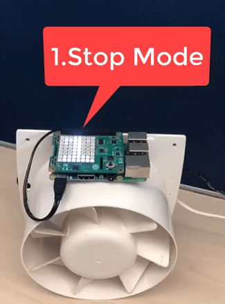
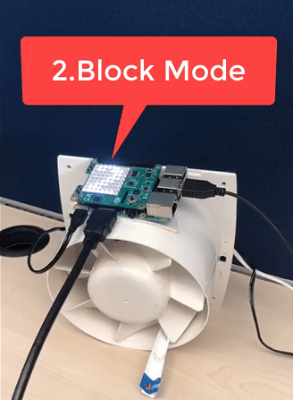
In this example, the operational state of the rotating device is divided into four modes: Stop, Block, Normal, and Rotor Imbalanced. This example uses a Sense HAT shield, which displays these operational modes on the 8x8 RGB LED display as 1, 2, 3, and 4, respectively. The Raspberry Pi determines the state by sensing the vibrations, using the Sense HAT LSM9DS1 IMU Sensor, in the X-, Y-, and Z-directions.

You can extract features such as mean, root mean square (RMS), and power spectral density from the vibration data of a rotating device, which are required for performing further data classification and developing a predictive model to identify the defined operational modes.

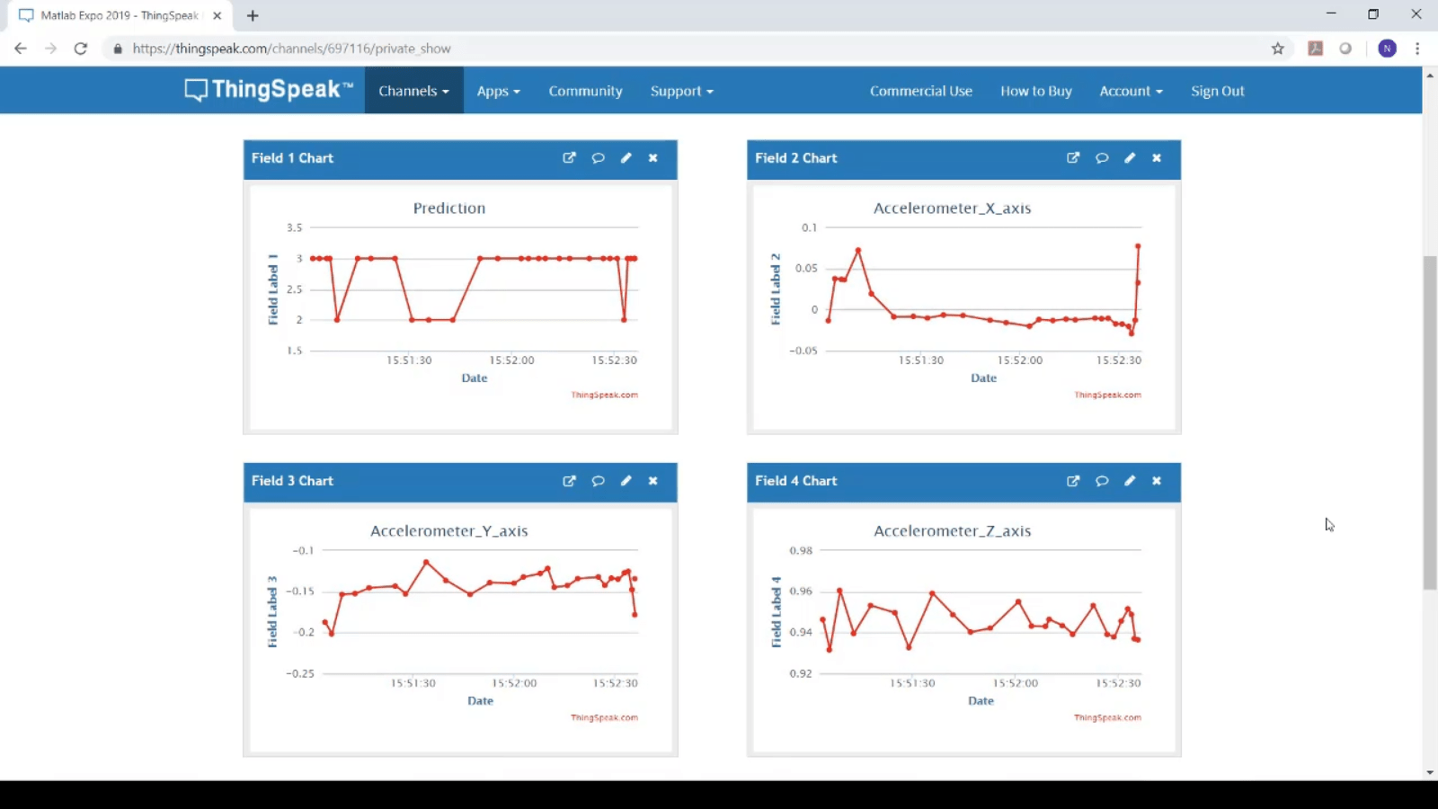
In addition to displaying the number representing the operational mode of the device on the 8x8 RGB LED Matrix, you can use the ThingSpeak platform to view the operational state in the cloud.

Prerequisites

For more information on how to use Simulink Support Package for Raspberry Pi Hardware, see Get Started with Simulink Support Package for Raspberry Pi Hardware.
For more information on using machine learning on embedded applications, see the Developing and Deploying Machine Learning Solutions for Embedded Applications video.

Required Hardware

Raspberry Pi board
Any device that contains moving parts. This example uses a rotating fan.
Sense HAT shield
Connecting wires
Any object for blocking the normal operational mode of a device. This example uses cardboard.
Adhesive or sticking tape

Hardware Setup

Connect the Sense HAT shield to the Raspberry Pi hardware board.
Place the entire hardware setup in a secure location on the rotating device. Use an adhesive or a piece of tape to secure the hardware board on top of the device. Ensure that no connecting wires create an obstacle while the device vibrates.

Prepare Data Set for Training Deep Learning Algorithm

This example uses a pretrained feature data set available in MATLAB®. To load the MAT file, run this command in the MATLAB Command Window.

load raspi_training_data_pdm.mat

Observe that the fullfeattable.mat file is loaded in the MATLAB Workspace. This MAT file contains a 283-by-34 matrix of features extracted for a fan. These features indicate what attributes these features measure (such as acceleration or vibration). They have been calculated using the raw X-, Y-, and Z-axes acceleration data values for the fan operating in four different modes.

Observe that the mean values are stored in columns 1 through 3, root mean square values in columns 4 through 6, and power spectral density values for each axis in columns 7 through 33. The 34th column defines the operational mode of the device. If you use this MAT file, continue from the Configure Simulink Model and Calibrate Parameters section. Alternatively, you can capture the acceleration data of any other rotating device using an IMU sensor. Follow these steps to capture and train acceleration data for any other rotating device using an IMU sensor.

A. Data Acquisition Using Accelerometer

B. Feature Extraction

C. Develop Predictive Model to Classify Data

Data Acquisition Using Accelerometer

You can use any IMU sensor to obtain acceleration data values along the X-, Y-, and Z-axes. This example uses the LSM9DS1 IMU Sensor.

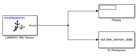
To save the acceleration data obtained from the IMU sensor in a MAT file, first create a new Simulink model. Then add these blocks to the model canvas.

1. LSM9DS1 IMU Sensor, from the Simulink Support Package for Raspberry Pi Hardware/Sense HAT library.

2. Display, from the Simulink/Dashboard library.

3. To Workspace, from Simulink/Sinks library.

Connect the Accel port of the LSM9DS1 IMU Sensor block to the input ports of the Display and To Workspace blocks.

Configure these parameters in the LSM9DS1 IMU Sensor Block Parameters dialog box.

1. Set the Board parameter to Pi 2 Model B.

2. Set the Active sensors parameter to Accelerometer.

3. Set the Sample time parameter to 0.02.

This sensor captures the acceleration data every 0.02 seconds. The Display block displays the 1-by-3 vector output for the acceleration data along the X-, Y-, and Z- axes.

Configure these parameters in the To Workspace Block Parameters dialog box.

1. Set the Variable Name parameter to raw_sensor_data.

2. Set the Save format parameter to Array.

3. Set the Save 2-D signals as parameter to 2-D array (concatenate along first dimension).

4. Set the Sample time parameter to 0.02.

On the Hardware tab of the Simulink model, in the Mode section, select Run on board and then click Monitor & Tune.

For capturing data in the Stop mode, ensure that the device is in the power OFF state. Similarly, for capturing data in the Normal mode, power ON the device. Use a piece of cardboard or any other object to block any moving part of the device while in the ON state. For the Rotor Imbalanced mode, you can move or shake the whole setup of the device.

Observe the acceleration data stored in the raw_sensor_data.mat file.

The LSM9DS1 IMU Sensor captures the acceleration data every 0.02 seconds. The X-, Y-, and Z-buffers store the 1-by-3 vector output for the acceleration data along the X-, Y-, and Z-axes.

Feature Extraction

Use the MATLAB code in the raspberrypi_pdm_extract_features.m function file to extract features from the raw acceleration data for the four modes of operation for your device. This function calculates the mean, root mean square (RMS), and power spectral density for the raw acceleration data and stores them in the adjacent columns of the raw_sensor_data.mat file. The function calculates these features for every 50 data sample values.

In this MATLAB function:

samplesPerObservation is the number of samples that the IMU sensor captures.
accx_mat, accy_mat, and accz_mat correspond to the input acceleration data received from the IMU sensor, for the X-, Y-, and Z-axes, respectively.
featmat corresponds to the entire feature data set.
feature1, feature2, and feature3 correspond to the mean values calculated for the X-, Y-, and Z-input acceleration data, respectively.

You can execute this MATLAB function for one operational mode at a time and capture the features. These features are stored in column 1 through 33 of the MAT file.

To capture the acceleration data in all the operational modes, run these commands in the MATLAB Command Window.

extracted_features = raspberrypi_pdm_extract_features(out,1); % stop mode
extracted_features = [extracted_features; raspberrypi_pdm_extract_features(out,2)]; %block mode
extracted_features = [extracted_features; raspberrypi_pdm_extract_features(out,3)]; % normal mode
extracted_features = [extracted_features; raspberrypi_pdm_extract_features(out,4)]; % rotor imabalance mode

Develop Predictive Model to Classify Data

The Classification Learner app helps you explore supervised machine learning using various classifiers. Using this app, you can explore your data, select features, specify validation schemes, train models, and assess results. You can perform automated training to search for the best classification model type of your application. You can perform supervised machine learning by supplying a known set of input data (observations or examples) and known responses to the data (such as labels or classes). You use this data to train a model that generates predictions for the response to new data. To use the model with new data, or to learn about programmatic classification, you can export the model to the workspace or generate MATLAB code to recreate the trained model. For more information, see the Classification Learner App (Statistics and Machine Learning Toolbox).

1. To open the Classification Learner app, enter classificationLearner in the MATLAB Command Window. You can also find the app on the Apps tab, under Machine Learning.

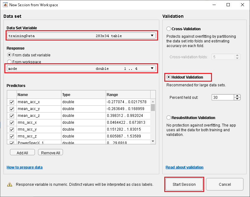
2. In the Classification Learner tab of the app, click New Session and select From Workspace. Ensure that the extracted_features.mat file is present in the MATLAB Workspace.

3. In the New Session from Workspace dialog box, select the extracted_features.mat file from the Data Set Variable list.

4. In the Response section, select From data set variable and select the response column of your MAT file from the drop-down. In this example, the name of the column is mode.

5. In the Validation section, select Holdout Validation. Select a percentage of the data to use as a validation set. The app trains a model on the training set and assesses its performance with the validation set. The model used for validation is based on only a portion of the data, so Holdout Validation is recommended only for large data sets. The final model is trained with the full data set. In this example, Percent held out is set to 30. This value indicates that 70% of the data is used for training the machine learning algorithm.

6. Click Start Session.

7. Before you train a classifier, the Scatter Plot shows the data. In the Plot section, select Data to plot only the data.

8. Choose features to plot using the X and Y lists under Predictors. Select predictor inputs that separate classes well by plotting different pairs of predictors on the scatter plot. For example, plotting the extracted_features.mat data, you can see that the RMS values of acceleration data along the Z-axis and the mean values of acceleration data along the Y-axis separate class 4, corresponding to the Rotor Imbalance mode. Plot other predictors to see if you can separate the other classes. You can add or remove predictors using the check boxes in the Classes section.

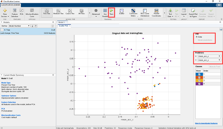
9. To create a classification model, on the Classification Learner tab, in the Model Type section, expand the gallery and select the type of model to train using the data. For this example, select Bagged Trees.

10. Click Train. The app generates a confusion matrix for the Bagged Trees model.

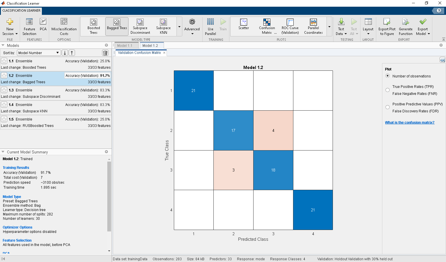
11. Select and train two or more models on the data, and observe the Accuracy (Validation) score for each model. Choose the best model among those you train by examining their performance in each class.

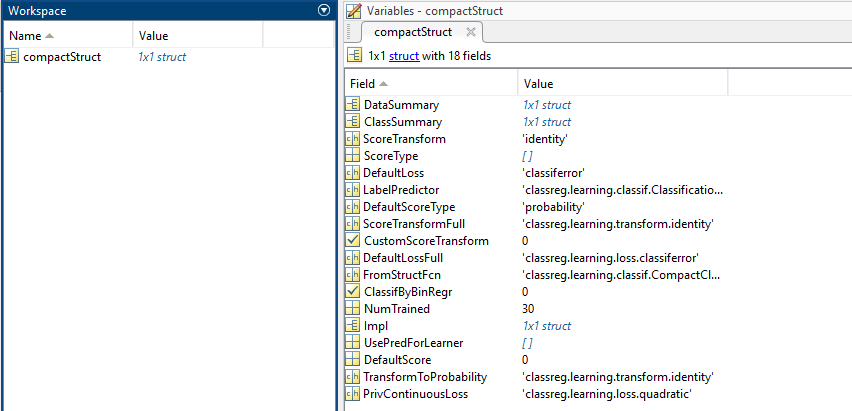
12. To export the model to the workspace, on the Classification Learner tab, in the Export section, click Export Model and select Export Compact Model. In the Export Model dialog box, enter the name of the workspace variable to which to export the model and click OK. In this example, variable name is ensembleclassifier. MATLAB creates an ensembleclassifier.mat file in the current directory of the example. This MAT file contains a structure that defines all the properties for the Bagged Trees classification model of the data trained using the Classification Learner app.

13. To save the ensembleclassifier variable in a MAT file, execute this command in the MATLAB Command Window.

save('ensembleclassifier.mat','ensembleclassifier')

Configure Simulink Model and Calibrate Parameters

Open the raspberrypi_predictiveMaintenance Simulink model.

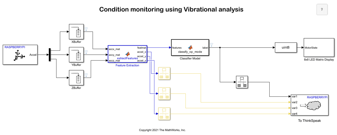
Configure these parameters in the X, Y, and Z Buffer (DSP System Toolbox) Block Parameters dialog box.

Set the Output buffer size parameter to 50.
Set the Buffer overlap parameter to 20.

Each buffer stores 50 data samples every 0.02 seconds corresponding to each axis.

The Rate Transition block transfers the calculated mean data from the accel_x, accel_y, and accel_z outputs of the extractFeatures MATLAB Function block, operating at one rate, to the inputs of the ThingSpeak Write block, operating at a different rate.

Configure these parameters in all the three Rate Transition Block Parameters dialog boxes.

Clear the Ensure deterministic data transfer (maximum delay) parameter.
Set Output port sample time to 1.

Double-click the MATLAB Function block and copy this code to the M file.

function label = classify_op_mode(features)
%%label = zeros(1,1);
   mdl = loadLearnerForCoder('raspi_trained_model_pdm.mat');
   label = predict(mdl,features);

end

The loadLearnerForCoder (Statistics and Machine Learning Toolbox) function loads the training model. Enter the name of the MAT file that you exported using the Classification Learner app as the argument for the loadLearnerForCoder function.

Cloud-Based Communication Using ThingSpeak

ThingSpeak™ cloud can help you view and monitor the health of a rotating device from a remote location. You can view the operational mode of the rotating device in ThingSpeak cloud. In this example, you use the ThingSpeak Write block view and monitor this data that it receives through the Rate Transition blocks:

label output from the Classifier Model MATLAB Function block
Mean of the X-axis acceleration data
Mean of the Y-axis acceleration data
Mean of the Z-axis acceleration data

Configure these parameters in the ThingSpeak Write Block Parameters dialog box.

Set Number of variables to send to 4.
Set Update interval to 0.1.
Select Print diagnostic messages.

Follow these steps to configure the ThingSpeak channel.

Login to your ThingSpeak account.
Select Channels > New Channel.
Enter a unique name in the Name parameter.
Enter a description for the channel in the Description parameter.
To display four parameters on the dashboard, select Field1, Field2, Field3, and Field4.
Enter the names Prediction, Accelerometer_X_axis, Accelerometer_Y_axis, and Accelerometer_Z_axis in the fields 1, 2, 3, and 4, respectively.
Click Save Channel. A dashboard screen is displayed with four sections.
On the dashboard, in the API Keys tab, copy the Key in the Write API Key section.
Paste this API key in the Write API Key parameter of the ThingSpeak Write block.

The Data Type Conversion block converts the label output received from the Classifier Model MATLAB Function block to the uint8 data type for further processing. Set Output data type to uint8.

Display Predictive Operational Mode on 8x8 RGB LED

The LED Output subsystem receives the MotorState input from the Classifier Model MATLAB Function block.

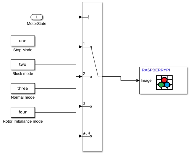
The MotorState input acts as a control input to the Multiport Switch block. The value at this port of the Multiport Switch block determines the output that is selected from one of the Constant blocks. The output is the predicted operational mode of the device and is displayed on the 8x8 RGB LED Matrix block.

Configure these parameters in the Multiport Switch Block Parameters dialog box.

Set Number of data ports to 4.
Set Diagnostic for default case to None.

Configure this parameter in the 8x8 RGB LED Matrix Block Parameters dialog box.

Set Mode to Display Image.

Deploy Simulink Model on Raspberry Pi Hardware

1. On the Hardware tab of the Simulink model, in the Mode section, select Run on board and then click Build, Deploy & Start.

2 Operate the device in four different modes of operation: Stop, Normal, Block, and Rotor Imbalanced. Observe that the 8x8 RGB LED Matrix displays the corresponding mode number.

3. Observe the four sections of the real-time data displayed on the ThingSpeak channel.