Batch Linearize Model at Multiple Operating Points Using Model Linearizer

To obtain linear models of your system under different operating conditions, you can interactively batch linearize your Simulink^® model at multiple operating points using Model Linearizer.

Alternatively, you can batch linearize your model programmatically. For more information, see Batch Linearize Model at Multiple Operating Points Using linearize Command and Vary Operating Points and Obtain Multiple Transfer Functions Using slLinearizer Interface.

Linearize at Multiple Trimmed Operating Points

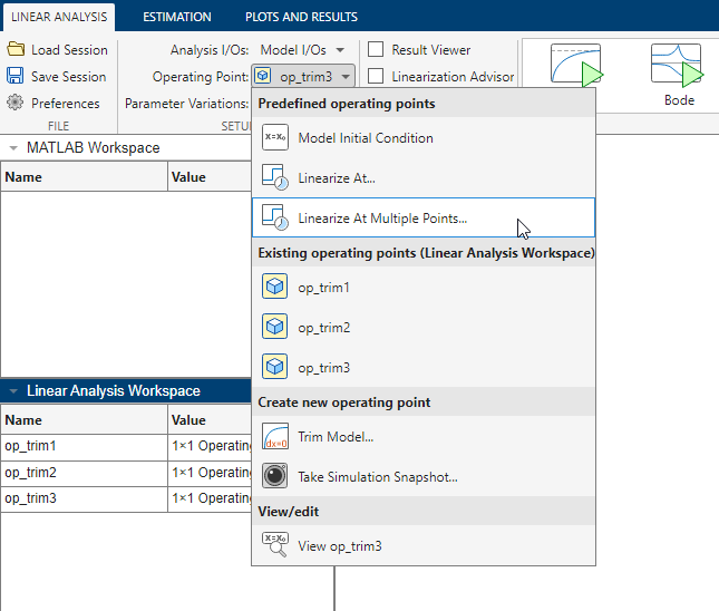
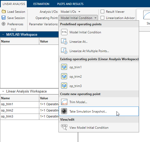
To linearize your model at multiple trimmed operating points, in Model Linearizer, on the Linear Analysis tab, select Operating Point > Linearize At Multiple Points.

Operating Point drop-down list open with the cursor over the Linearize At Multiple Points option.

In the Specify multiple operating points dialog box, the table lists all available operating points in the Model Linearizer Linear Analysis Workspace or the MATLAB^® workspace.

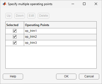
Specify multiple operating points dialog box with all three models in the table selected in the leftmost column.

In the Selected column, select the operating points at which you want to linearize the model.

To reorder operating points in the list, use the Up and Down buttons. Model Linearizer places linearized models in an array corresponding to the order of the operating points in this list.

Click OK.

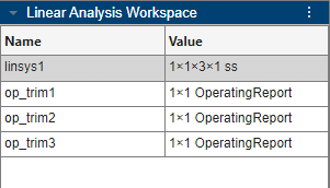
To linearize the model, on the Linear Analysis tab, in the Linearize gallery, select a plot type. The app linearizes the model at the specified operating points, adds the resulting model array to the Linear Analysis Workspace, and plots the selected analysis plot.

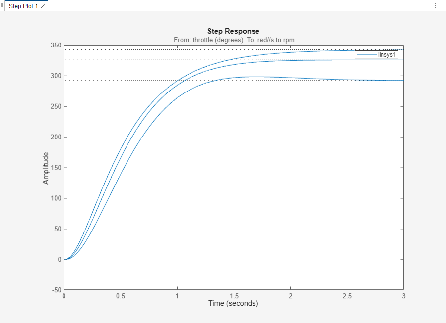
Linear Analysis Workspace section showing linsys1, which is a 1-by-1-by-3-by-1 stat-space model array.

The following figure shows a step plot for a model linearized at three different operating points.

Step responses for three models within the linsys1 model array.

Linearize at Multiple Simulation Snapshots

If you know the approximate time in a simulation when your model reaches the neighborhood of a steady-state operating point, you can use simulation to get state values to use as the initial conditions for numerical optimization.

In Model Linearizer, on the Linear Analysis tab, select Operating Point > Take Simulation Snapshot.

Operating Point drop-down list open with the cursor over the Take Simulation Snapshot option.

To trim the model at multiple snapshot times, specify an array of times in the Enter snapshot times to linearize dialog box. For example, the following figure specifies snapshot times of 5 and 10 seconds.

Enter snapshot times to linearize with [5 10] specified in the text field.

Click Take Snapshots.

The app simulates the model and uses the model states at each snapshot time as the initial condition for an operating point search. The resulting operating points are added to the Linear Analysis Workspace in an operating point array.

Blocks with Internal State Representations

If your model contains blocks with internal state representations, the operating points computed from initial snapshots do not contain the corresponding internal states. As a result, the computed operating points might not be accurate linear representations of the model. For more information, see Handle Blocks with Internal State Representation.

Instead of computing operating points at the simulation snapshots, you can simulate the model up to the snapshot times and linearize the model at the snapshots themselves.

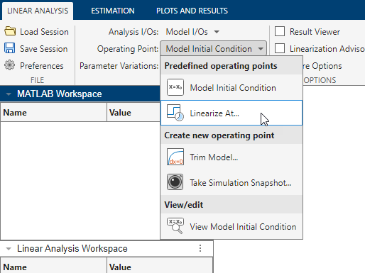
In Model Linearizer, on the Linear Analysis tab, select Operating Point > Linearize At.

Operating Point drop-down list open with the cursor over the Linearize At option.

In the Enter snapshot times to linearize dialog box, specify an array of snapshot times. For example, the following figure specifies snapshot times of 5 and 10 seconds.

Enter snapshot times to linearize with [5 10] specified in the text field.

Click OK.

When you subsequently linearize the model, the app simulates the model and computes a linear representation based on the state of the model at each snapshot time, including any internal states.