Batch Linearize Model at Multiple Operating Points Using linearize Command
This example shows how to use the linearize command to batch linearize a model at varying operating points.
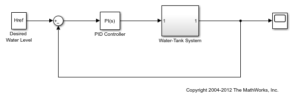
Obtain the plant transfer function, modeled by the Water-Tank System block, for the watertank model. You can analyze the batch linearization results to study the operating point effects on the model behavior.
Open the model.
open_system('watertank')

Specify the linearization I/Os.
ios(1) = linio('watertank/PID Controller',1,'input');
ios(2) = linio('watertank/Water-Tank System',1,'openoutput');
ios(2) specifies an open-loop output point; the loop opening eliminates the effects of feedback.
You can linearize the model using trimmed operating points, the model initial condition, or simulation snapshot times. For this example, linearize the model at specified simulation snapshot times.
ops_tsnapshot = [1,20];
Obtain the transfer function for the Water-Tank System block, linearizing the model at the specified operating points.
T = linearize('watertank',ios,ops_tsnapshot);
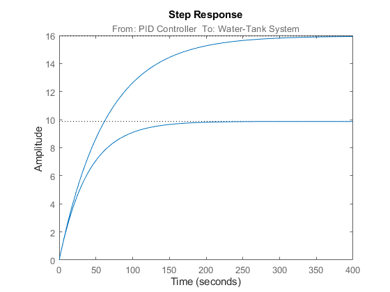
T is a 2 x 1 array of linearized continuous-time state-space models. The software computes the T(:,:,1) model by linearizing watertank at ops_tsnapshot(1), and T(:,:,2) by linearizing watertank at ops_tsnapshot(2).
Use Control System Toolbox™ analysis commands to examine the properties of the linearized models in T. For example, examine the step response of the plant at both snapshot times.
stepplot(T)

See Also
linearize | findop | linio | stepplot
Topics
- watertank Simulink Model
- Batch Compute Steady-State Operating Points for Multiple Specifications
- Vary Operating Points and Obtain Multiple Transfer Functions Using slLinearizer Interface
- Batch Linearize Model for Parameter Variations at Single Operating Point
- Analyze Command-Line Batch Linearization Results Using Response Plots