Time-Domain Specifications

Step Command Following

The TuningGoal.StepTracking requirement specifies how the tuned closed-loop system should respond to a step input. You can specify the desired response either in terms of first- or second-order characteristics, or as an explicit reference model. This requirement is satisfied when the relative gap between the actual and desired responses is small enough in the least-squares sense. For example,

R1 = TuningGoal.StepTracking('r','y',0.5);

stipulates that the closed-loop response from r to y should behave like a first-order system with time constant 0.5, while

R2 = TuningGoal.StepTracking('r','y',zpk(2,[-1 -2],-1));

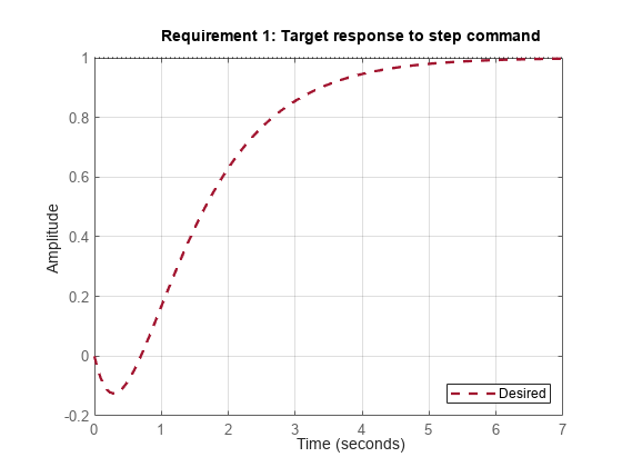
specifies a second-order, non-minimum-phase behavior. Use viewGoal to visualize the desired response.

viewGoal(R2)

This requirement can be used to tune both SISO and MIMO step responses. In the MIMO case, the requirement ensures that each output tracks the corresponding input with minimum cross-couplings.

Step Disturbance Rejection

The TuningGoal.StepRejection requirement specifies how the tuned closed-loop system should respond to a step disturbance. You can specify worst-case values for the response amplitude, settling time, and damping of oscillations. For example,

R1 = TuningGoal.StepRejection('d','y',0.3,2,0.5);

limits the amplitude of $$y(t)$$ to 0.3, the settling time to 2 time units, and the damping ratio to a minimum of 0.5. Use viewGoal to see the corresponding time response.

viewGoal(R1)

You can also use a "reference model" to specify the desired response. Note that the actual and specified responses may differ substantially when better disturbance rejection is possible. Use the TuningGoal.Transient requirement when a close match is desired. For best results, adjust the gain of the reference model so that the actual and specified responses have similar peak amplitudes (see TuningGoal.StepRejection documentation for details).

Transient Response Matching

The TuningGoal.Transient requirement specifies the transient response for a specific input signal. This is a generalization of the TuningGoal.StepTracking requirement. For example,

R1 = TuningGoal.Transient('r','y',tf(1,[1 1 1]),'impulse');

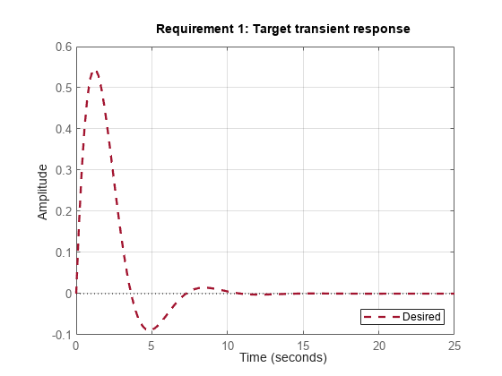
requires that the tuned response from $$r$$ to $$y$$ look like the impulse response of the reference model $$1/(s^2+s+1)$$.

viewGoal(R1)

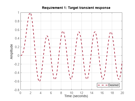
The input signal can be an impulse, a step, a ramp, or a more general signal modeled as the impulse response of some input shaping filter. For example, a sine wave with frequency $${\omega }_0$$ can be modeled as the impulse response of $${\omega }_0^2/(s^2+{\omega }_0^2)$$.

w0 = 2;
F = tf(w0^2,[1 0 w0^2]);  % input shaping filter
R2 = TuningGoal.Transient('r','y',tf(1,[1 1 1]),F);
viewGoal(R2)

LQG Design

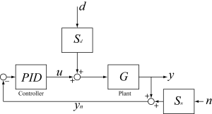
Use the TuningGoal.LQG requirement to create a linear-quadratic-Gaussian objective for tuning the control system parameters. This objective is applicable to any control structure, not just the classical observer structure of LQG control. For example, consider the simple PID loop of Figure 2 where $$d$$ and $$n$$ are unit-variance disturbance and noise inputs, and $$S_d$$ and $$S_n$$ are lowpass and highpass filters that model the disturbance and noise spectral contents.

Figure 2: Regulation loop.

To regulate $$y$$ around zero, you can use the following LQG criterion:

The first term in the integral penalizes the deviation of $$y(t)$$ from zero, and the second term penalizes the control effort. Using systune, you can tune the PID controller to minimize the cost $$J$$. To do this, use the LQG requirement

Qyu = diag([1 0.05]);  % weighting of y^2 and u^2
R4 = TuningGoal.LQG({'d','n'},{'y','u'},1,Qyu);