Tune Field-Oriented Controllers Using SYSTUNE

Field-Oriented Control

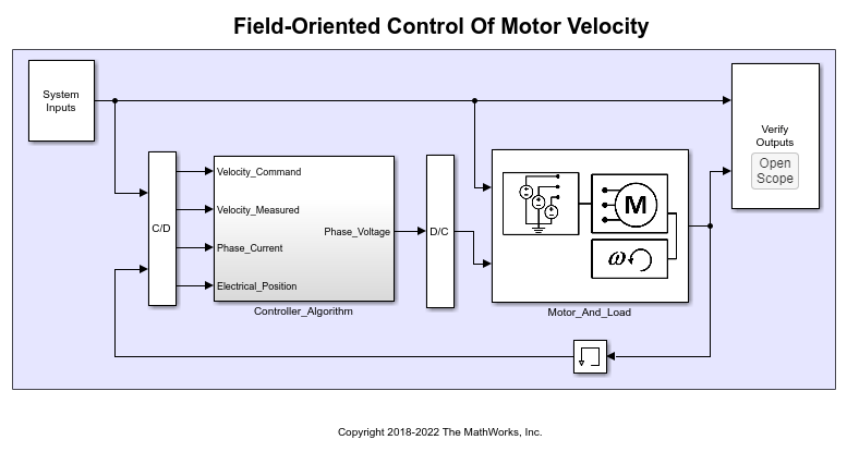
In this example, field-oriented control (FOC) for a permanent magnet synchronous machine (PMSM) is modeled in Simulink® using Simscape™ Electrical™ components.

mdl = 'scdfocmotorSystune';
open_system(mdl)
SignalEditorPath = [mdl,'/System_Inputs/Reference_System_Inputs'];

Field-oriented control controls 3-phase stator currents as a vector. FOC is based on projections, which transform a 3-phase time-dependent and speed-dependent system into a two-coordinate time-invariant system. These transformations are the Clarke Transformation, Park Transformation, and their respective inverse transforms. These transformations are implemented as blocks within the Controller_Algorithm subsystem.

The advantages of using FOC to control AC motors include:

The Controller_Algorithm subsystem contains all three PI controllers. The outer-loop PI controller regulates the speed of the motor. The two inner-loop PI controllers control the d-axis and q-axis currents separately. The command from the outer loop PI controller directly feeds to the q-axis to control torque. The command for the d-axis is zero for PMSM because the rotor flux is fixed with a permanent magnet for this type of AC motor.

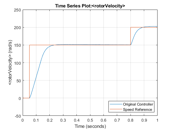
Before tuning controllers, examine the speed responses with the original controllers, and save the simulation results to a MAT file, SystunedSpeed.mat. The existing speed PI controller has gains of P = 0.08655 and I = 0.1997. The current PI controllers both have gains of P = 1 and I = 200.

scdfocmotorSystuneOriginalResponse

Plot the speed response with the original controllers. The plots exhibit steady-state errors and relatively slow transient behavior. You can tune the controllers to achieve a better performance.

figure
plot(logsout_original_oneside{2}.Values);
hold on
plot(logsout_original_oneside{1}.Values);
legend('Original Controller','Speed Reference','Location','southeast');
grid on
hold off

figure
plot(logsout_original_twoside{2}.Values);
hold on
plot(logsout_original_twoside{1}.Values);
legend('Original Controller','Speed Reference','Location','northeast');
grid on
hold off

Collect Frequency Response Data

To collect frequency response data, find an operating point at a speed of 150 rad/sec, specify linear analysis points, define input signals, and estimate the frequency response.

Disconnect the original controllers, and simulate the open-loop system model with VD and VQ commands. To reach the operating point, specify initial voltages of -0.1 V for VD and 3.465 V for VQ using the ctrlIniValues structure. Constant voltage command blocks are connected by setting switch signals in the switchIniValue structure.

switchIniValue.openLoopD = 1;
switchIniValue.openLoopQ = 1;
ctrlIniValues.voltageD = -0.1;
ctrlIniValues.voltageQ = 3.465;

Capture a simulation snapshot at 3 sec as the operating point for frequency response estimation.

set_param(SignalEditorPath,'ActiveScenario',...
    'Test_Case_150_rad_sec_Steady_state');
op = findop(mdl,3);

Use the simulation snapshot operating point as the initial condition of the model. Change the model initial values in the ctrlIniValues structure to be at this steady state. For the d-axis current controller, the current ID is 0 A. For the q-axis current controller, the current IQ is 0.1 A. For the outer-loop speed controller, the reference current is 0.122 A and the speed is at 150 rad/s. For the PMSM plant, set the rotor velocity in the pmsm structure to 150 rad/s.

set_param(mdl,'LoadInitialState','on');
set_param(mdl,'InitialState','getstatestruct(op)');
ctrlIniValues.currentDIC = 0;
ctrlIniValues.currentQIC = 0.1;
ctrlIniValues.speedIC = 150;
ctrlIniValues.speedCurrent = 0.122;
pmsm.RotorVelocityInit = 150;

Add linear analysis points to the model for frequency response estimation. Add open-loop input points to VD and VQ. Add open-loop output points to ID, IQ, and speed. In addition, add a loop break analysis point to the speed measurement.

io = getlinio(mdl);

Define input sinestream signal from 10 to 10,000 rad/s with a fixed sample time of 4e-6 s, that is, the sample time of the current control loop sampleTime.CurrentControl. The sinestream signal magnitude is 0.25 V. This magnitude ensures that the plant is properly excited within the saturation limit. If the excitation amplitude is either too large or too small, it produces inaccurate frequency response estimation results.

in = frest.createFixedTsSinestream(sampleTime.CurrentControl,{10,1e4});
in.Amplitude = 0.5;

Estimate the frequency response at the specified steady state operating point op, using the linear analysis points in io and the input signals in in. After finishing the frequency response estimation, modify the input and output channel names in the resulting model, and plot the frequency response.

estsys = frestimate(mdl,op,io,in);
estsys.InputName = {'Vd','Vq'};
estsys.OutputName = {'Id','Iq','speed'};
figure
bode(estsys,'.')

Tune Control System Using systune

Obtain a state-space linear system model from the frequency response estimation result. Using an option set for the ssest function, set the numerical search method used for this iterative parameter estimation as the Levenberg-Marquardt least-squares search. Estimate a state-space model with four states and a period of 4e-6 seconds. This step requires System Identification Toolbox™ software.

optssest = ssestOptions('SearchMethod','lm');
optssest.Regularization.Lambda = 0.1;
sys_singletune = ssest(estsys,4,'Ts',sampleTime.CurrentControl,optssest);

In order to tune all three PI controllers in the PMSM FOC model, construct a control system as shown in the following block diagram.

Define three tunable discrete-time PID blocks and their I/Os for d-axis current control, q-axis current control, and speed control. The sample times of these discrete-time PID controllers must be consistent, which is the same as the current control loop sample time. To ensure a better approximation of faster controllers as compared to the original slower controllers, set the discrete integrator formula for each PID controller to 'Trapezoidal'.

Cd = tunablePID('Cd','pi',sampleTime.CurrentControl);
Cd.IFormula = 'Trapezoidal';
Cd.u = 'Id_e';
Cd.y = 'Vd';

Cq = tunablePID('Cq','pi',sampleTime.CurrentControl);
Cq.IFormula = 'Trapezoidal';
Cq.u = 'Iq_e';
Cq.y = 'Vq';

Cspeed = tunablePID('Cspeed','pi',sampleTime.CurrentControl);
Cspeed.IFormula = 'Trapezoidal';
Cspeed.u = 'speed_e';
Cspeed.y = 'Iq_ref';

Create three summing junctions for the inner and outer feedback loops.

sum_speed = sumblk('speed_e = speed_ref - speed');
sum_id = sumblk('Id_e = Id_ref - Id');
sum_iq = sumblk('Iq_e = Iq_ref - Iq');

Define inputs, outputs, and analysis points for controller tuning.

input = {'Id_ref','speed_ref'};
output = {'Id','Iq','speed'};
APs = {'Iq_ref','Vd','Vq','Id','Iq','speed'};

Finally, assemble the complete control system, ST0, using these components.

ST0 = connect(sys_singletune,Cd,Cq,Cspeed,sum_speed,sum_id,sum_iq,input,output,APs);

Define tuning goals, including tracking and loop shape goals to ensure command tracking, as well as gain goals to prevent saturations. For the speed controller, set the tracking bandwidth to 150 rad/s. This bandwidth is used in both the tracking and loop shape goals. Additionally, set the DC error to 0.001 to reflect a maximum steady-state error of 0.1%. Set the peak error to 10. For the d-axis current controller, set the tracking bandwidth to 2500 rad/s, which is much faster than the outer-loop speed controller. To prevent saturating controllers, specify goals to constrain the gains for all three controllers.

TR1 = TuningGoal.Tracking('speed_ref','speed',2/150,0.001,10);
TR2 = TuningGoal.Tracking('Id_ref','Id',2/2500);
LS1 = TuningGoal.LoopShape('Id',2500);
LS2 = TuningGoal.LoopShape('speed',150);
MG1 = TuningGoal.Gain('speed_ref','Iq_ref',2);
MG2 = TuningGoal.Gain('speed_ref','Vq',50);
MG3 = TuningGoal.Gain('Id_ref','Vd',20);

Tune all three PI controllers using systune with all tuning goals based on the constructed model ST0. To increase the likelihood of finding parameter values that meet all design requirements, set options for systune to run five additional optimizations starting from five randomly generated parameter values.

opt = systuneOptions('RandomStart',5);
rng(2)
[ST1,fSoft] = systune(ST0,[TR1,TR2,LS1,LS2,MG1,MG2,MG3],opt);

Final: Soft = 1.01, Hard = -Inf, Iterations = 142
       Some closed-loop poles are marginally stable (decay rate near 1e-07)
Final: Soft = 1.01, Hard = -Inf, Iterations = 80
       Some closed-loop poles are marginally stable (decay rate near 1e-07)
Final: Soft = 1.01, Hard = -Inf, Iterations = 55
Final: Soft = 1.01, Hard = -Inf, Iterations = 60
Final: Soft = 1.01, Hard = -Inf, Iterations = 55
Final: Soft = 1.01, Hard = -Inf, Iterations = 45
       Some closed-loop poles are marginally stable (decay rate near 1e-07)

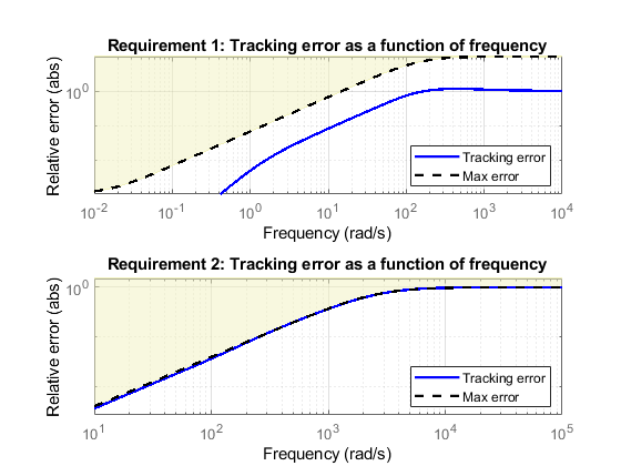
After finding a solution using systune, show how tuning goals are met in the tuned model ST1. Show the tracking, loop shape, and gain tuning goals separately. Dashed lines in the following figures represent tuning goals and solid lines are the result of the tuned controllers.

figure
viewGoal([TR1,TR2],ST1)
figure
viewGoal([LS1,LS2],ST1)
figure
viewGoal([MG1,MG2,MG3],ST1)

After verifying tuning goals, extract controller parameters from the tuned model ST1. Use tuned PI controller parameters to update the workspace parameters for the PI controller blocks.

Cd = getBlockValue(ST1,'Cd');
Cq = getBlockValue(ST1,'Cq');
Cspeed = getBlockValue(ST1,'Cspeed');

The d-axis current PI controller has tuned gains:

paramCurrentControlPD = Cd.Kp
paramCurrentControlID = Cd.Ki

paramCurrentControlPD =

    2.6633


paramCurrentControlID =

   2.4342e+03

The q-axis current PI controller has tuned gains:

paramCurrentControlPQ = Cq.Kp
paramCurrentControlIQ = Cq.Ki

paramCurrentControlPQ =

    5.3736


paramCurrentControlIQ =

  670.7248

The speed PI controller has tuned gains:

paramVelocityControlTuneP = Cspeed.Kp
paramVelocityControlTuneI = Cspeed.Ki

paramVelocityControlTuneP =

    0.3497


paramVelocityControlTuneI =

    0.0628

After tuning all three controllers together using systune, the controller gains are significantly different from the original values. The PID controller in the speed control loop has a different sample time, which is 0.001 second. The tuned result uses a different sample time of 4e-6 second but the controller gains are the same. To make sure controller performances are identical with different sample times, the discrete integrator format of the PID controllers is 'Trapezoidal' in this example.

Validate Tuned Controller

Examine the performances using the tuned controller gains. First, initialize the model to its zero initial conditions using ctrlIniValues. Connect the PID controller blocks by setting switch signals in the switchIniValue and set proper initial conditions for the PMSM plant model.

switchIniValue.openLoopQ = 0;
switchIniValue.openLoopD = 0;
ctrlIniValues.currentDIC = 0;
ctrlIniValues.voltageD = 0;
ctrlIniValues.currentQIC = 0;
ctrlIniValues.voltageQ = 0;
ctrlIniValues.speedIC = 0;
ctrlIniValues.speedCurrent = 0;
pmsm.RotorVelocityInit = 0;
set_param(mdl,'LoadInitialState','off')

Configure the model to use a one-sided speed command signal and simulate the model. Show the speed response of the model to the one-sided speed command that rises from 0 rad/s to 150 rad/s at 0.05 s, and then to 200 rad/s at 0.8 s. Save the simulation result to logsout_tuned_oneside in the MAT file, SystunedSpeed.mat.

set_param(SignalEditorPath,'ActiveScenario','Test_Case_150_rad_sec_No_load');
sim(mdl);
logsout_tuned_oneside = logsout;
save('SystunedSpeed','logsout_tuned_oneside','-append')

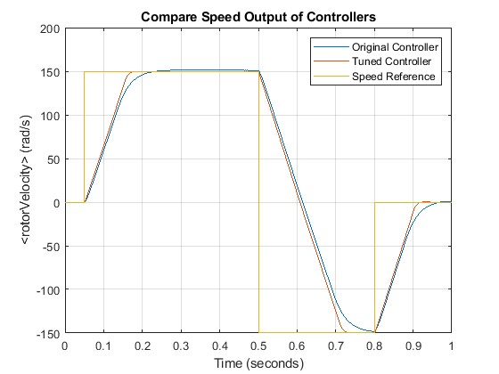
Configure the model to use a two-sided speed command signal and simulate the model. Show the speed response of the model to the two-sided speed command that rises from 0 rad/s to 150 rad/s at 0.05 s, reverses direction at 0.5 s and then back to 0 rad/s at 0.8 s. Save the simulation result to logsout_tuned_twoside in the MAT file, SystunedSpeed.mat.

set_param(SignalEditorPath,'ActiveScenario','Test_Case_1_150_rad_sec_No_load');
sim(mdl);
logsout_tuned_twoside = logsout;
save('SystunedSpeed','logsout_tuned_twoside','-append')

Compare the motor speed responses between the existing controller gains and the tuned result. The speed responses are shown side-by-side over the one-second simulation. The speed response follows more closely to the step command. The steady-state error also decreases after the PI controllers are tuned with systune.

scdfocmotorSystunePlotSpeed

After tuning the controllers, the motor response improves with faster transient response and smaller steady-state error under both types of speed commands.

bdclose(mdl)