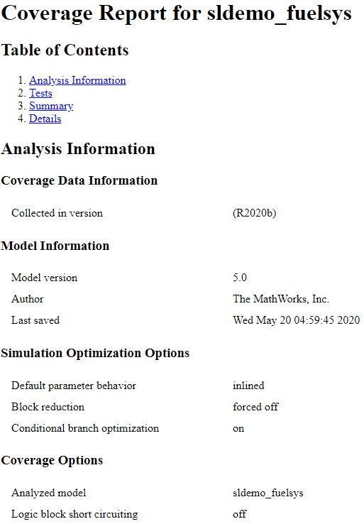
顶层模型覆盖率报告
如果您使用运行按钮分析模型的覆盖率,Simulink® Coverage™ 将为名为 model_name_cov.html
要访问 sldemo_fuelsys 模型,请在 MATLAB® 命令行窗口中执行以下命令:
openExample('sldemo_fuelsys');分析信息
分析信息部分包含正在分析的模型的基本信息:
覆盖率数据信息
模型信息
框架信息(如果您从 Simulink Test™ 框架录制覆盖率则会出现)
仿真优化选项
覆盖率选项
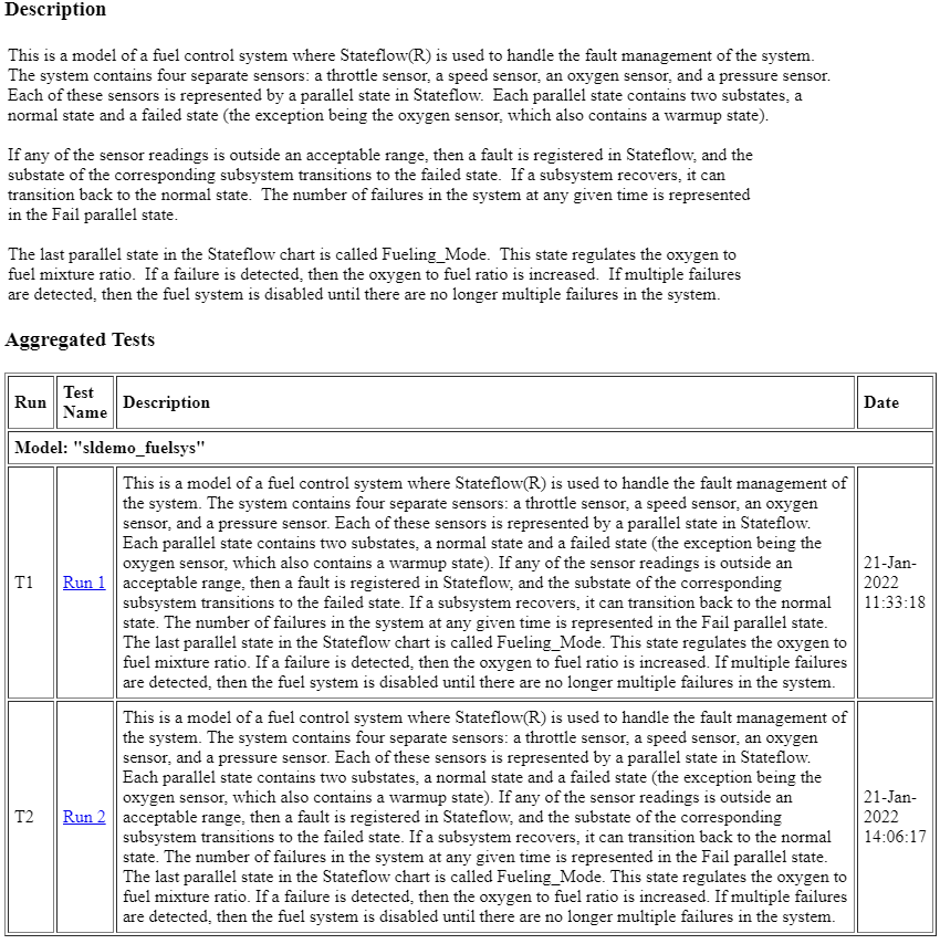
聚合测试
如果您执行以下操作,则会出现聚合测试部分:
通过 Simulink Test 管理器记录至少两个测试用例的聚合覆盖率结果,并针对聚合结果生成覆盖率报告,或者
在结果资源管理器中生成累计覆盖率结果的覆盖率报告。
如果您通过 Simulink Test 管理器运行测试用例,则聚合测试部分将链接到 Simulink Test 管理器中的相关测试用例。
如果您通过结果资源管理器聚合测试用例结果,则聚合的测试部分将链接到结果资源管理器中相应的 cvdata 节点。
对于聚合测试部分中的每次运行,都有一个指向 Simulink Test 管理器或结果资源管理器中相应结果的链接。
聚合单元测试
如果您记录一个或多个子系统框架的覆盖率,则“聚合测试”部分会列出每个单元测试运行,而“描述”部分会显示对聚合覆盖率数据的描述。您可以前往覆盖率结果浏览器并点击当前累积数据来查看和编辑此描述。
每个在测单元都会收到一个序数 n,在测单元的每个测试都会收到一个序数 m,格式为 Un.m。
覆盖率摘要
覆盖率摘要包含两个小节:
测试 - 每个测试用例的仿真开始和停止时间以及仿真之前的任何设置命令。每个测试用例的标题包括使用
cvtest命令指定的任何测试用例标签。仅当报告不包含 聚合测试 部分时才显示此部分。摘要 - 子系统结果的摘要。要查看特定子系统的详细结果,请在“摘要”子部分中点击子系统名称。
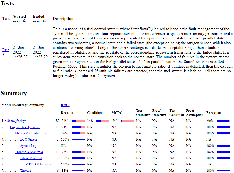
摘要部分包含每个请求的覆盖率度量的一列,即使对于那些不适用于所分析的模型或模型对象的度量也是如此。例如,在 sldemo_fuelsys 模型中,如果您选择目标和约束覆盖率度量,您将获得标题为测试目标、证明目标、测试条件和证明假设的列,即使该模型不包含 Simulink Coverage 可以针对这些度量进行分析的模块。
详细信息
详细信息部分报告详细的模型覆盖率结果。详细报告的每个部分总结了测试模型中每个对象的度量的结果:
您还可以按如下方式访问模型元素“详细信息”子部分:
右键点击 Simulink 元素。
在上下文菜单中,选择 覆盖率 > 报告。
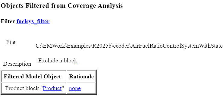
从覆盖率分析中滤除的对象
从覆盖率分析中滤除的对象部分列出了模型中从覆盖率记录中滤除的对象,以及为滤除这些对象指定的理由。如果过滤器规则指定过滤某种类型的所有模块,则所有这些模块都会在此处列出。
在下图中,名为 Product 的产品模块通过排除规则被滤除了。覆盖率报告显示覆盖率过滤器的名称、完整路径和文件名。它还会显示过滤器描述、被滤除的模块列表以及用于滤除这些模块的理由。过滤后的模型对象表格还会链接至该模块。点击链接可在模型中导航至该模块,系统用蓝色边框将其突出显示。点击筛选器名称或“理由”列中的链接,将打开从覆盖率结果浏览器到过滤器编辑器的窗格并显示筛选规则。
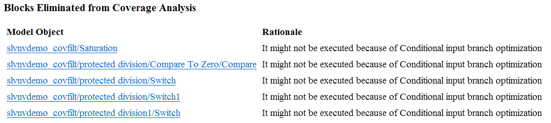
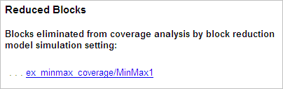
已从覆盖率分析中消除的模块
已从覆盖率分析中消除的模块部分列出了可能存在覆盖率缺失或因优化(如条件输入分支优化或模块简化)而未纳入覆盖率分析的每个模块。有关详细信息,请参阅Simulink 优化和模型覆盖率。
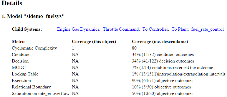
模型详细信息
详细信息部分包含整个模型的结果摘要,后面是元素列表。点击模型元素名称即可查看其覆盖率结果。
下图显示了 sldemo_fuelsys 示例模型的详细信息部分。
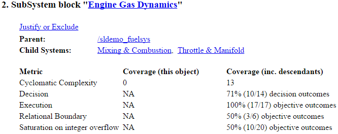
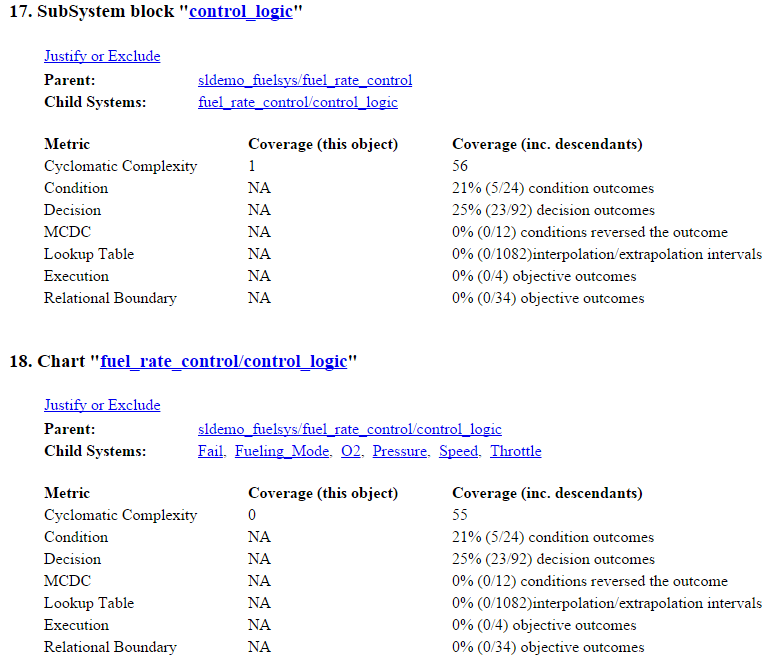
子系统详细信息
每个子系统详细信息部分包含子系统的测试覆盖率结果摘要及其所包含的子系统的列表。概述之后是模块、图和 MATLAB 函数部分,每个包含子系统中决策点的对象对应一个部分。
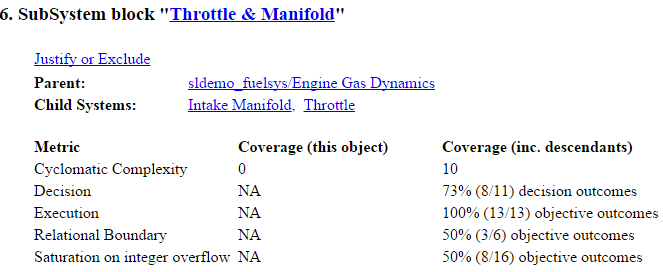
下图显示了 sldemo_fuelsys 示例模型中发动机气体动力学子系统的覆盖率结果。
模块详细信息
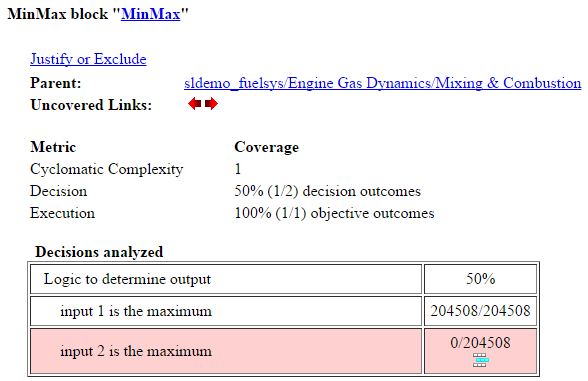
下图显示了 sldemo_fuelsys 示例模型中发动机气体动力学子系统的混合和燃烧子系统中 MinMax 模块的决策覆盖率结果。
未覆盖的链接元素首先出现在模型层次结构中未达到 100% 覆盖率的第一个模块的“模块详细信息”部分中。第一个未覆盖的链接元素有一个箭头,该箭头链接到下一个未达到 100% 覆盖率的模块的报告中“模块详细信息”部分。
未达到 100% 覆盖率的后续模块具有指向前一个和下一个未达到 100% 覆盖率的模块的报告中“模块详细信息”部分的链接。
图详细信息
下图显示了 control_logic 示例模型中 Stateflow® 图 sldemo_fuelsys 的覆盖率结果。
有关 Stateflow 图及其对象的模型覆盖率报告的更多信息,请参阅Stateflow 图的模型覆盖率。
MATLAB 函数和 Simulink Design Verifier 函数的覆盖率详细信息
默认情况下,Simulink Coverage 记录模型中所有 MATLAB 函数的覆盖率。MATLAB 函数位于 MATLAB Function 模块、Stateflow 图或外部 MATLAB 文件中。
注意
有关外部 MATLAB 文件的覆盖率报告的详细示例,请参阅外部 MATLAB 文件覆盖率报告。
要记录由 MATLAB 函数调用的 sldv.* 函数的 Simulink Design Verifier™ 覆盖率,以及任何 Simulink Design Verifier 模块,请在配置参数对话框的覆盖率窗格中选择目标和约束。
以下示例显示了调用四个 Simulink Design Verifier 函数的 MATLAB 函数、hFcnsInExternalEML 的覆盖率详细信息。在此示例中,hFcnsInExternalEML 的代码位于外部文件中。
此示例还显示了以下函数的 Simulink Design Verifier 覆盖率详细信息:
sldv.assume(Simulink Design Verifier)sldv.condition(Simulink Design Verifier)sldv.prove(Simulink Design Verifier)sldv.test(Simulink Design Verifier)
在覆盖率结果中,达到 100% 覆盖率的代码为绿色。覆盖率低于 100% 的代码为红色。
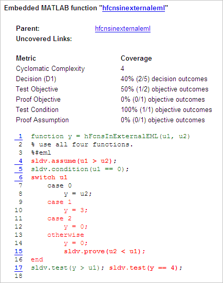
hFcnsInExternalEML 函数和 sldv.* 调用的覆盖率是:
第 1 行,
hFcnsInExternalEML的函数声明为绿色,因为仿真至少执行该函数一次。fcn在仿真中调用hFcnsInExternalEML11 次。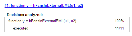
第 4 行,
sldv.assume(u1 > u2),实现 0% 覆盖率,因为u1 > u2从未被评估为 true。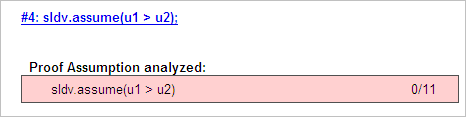
第 5 行
sldv.condition(u1 == 0)实现了 100% 的覆盖率,因为u1 == 0至少在一个时间步内计算为 true。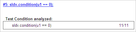
第 6 行
switch u1实现了 25% 的覆盖率,因为switch语句中的四个结果中只有一个 (case 0) 在仿真期间发生。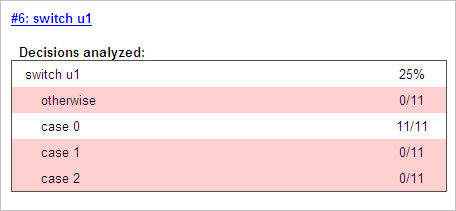
第 17 行,
sldv.test(y > u1); sldv.test (y == 4)实现 50% 的覆盖率。第一个sldv.test调用实现了 100% 的覆盖率,但是第二个sldv.test调用实现了 0% 的覆盖率。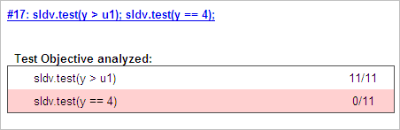
有关 MATLAB 函数覆盖率的更多信息,请参阅MATLAB 函数的模型覆盖率。
有关 Simulink Design Verifier 函数覆盖率的更多信息,请参阅目标和约束覆盖率。
需求测试详细信息
如果您在 Simulink Test 中运行至少两个与 Requirements Toolbox™ 中的需求相关联的测试用例,则聚合覆盖率报告会详细说明模型元素、测试用例和链接需求之间的联系。
需求测试详细信息部分包括:
已实现的需求 - 哪些需求与模型元素相关。
通过测试验证 - 哪些测试验证了需求。
关联的运行 - 哪些运行与每个验证测试相关。

有关如何在覆盖率报告中将覆盖率结果追踪到需求的示例,请参阅追踪覆盖率结果是否符合需求。
模型覆盖率报告中的圈复杂度
您可以指定模型覆盖率报告在报告的两个位置包含圈复杂度数字:
摘要部分包含模型层次结构中每个对象的圈复杂度数字。对于子系统或 Stateflow 图,该数字包括其所有后代的圈复杂度数字。
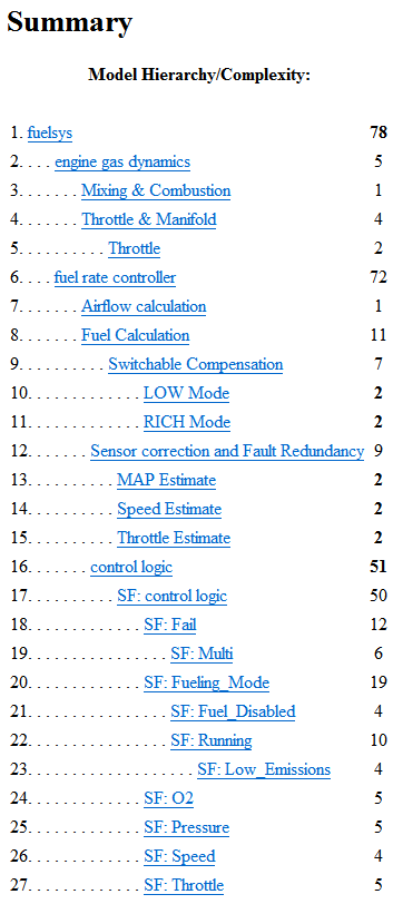
每个对象的详细信息部分列出了所有单个对象的圈复杂度数字。
分析的执行
分析的执行表显示模块在仿真期间执行的时间步数占仿真中的总时间步数。如果模块在至少一个时间步内执行,则覆盖率报告显示模块执行覆盖率完全满足。
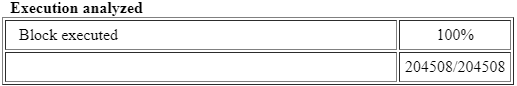
在图像中,Simulink Coverage 报告了 100% 的模块执行覆盖率,其中该模块在 204,508 个时间步中的 204,508 个时间步内执行。
已分析决策
分析的决策表列出了决策的可能结果以及每次测试仿真中该结果出现的次数。未发生的结果以红色突出显示的表行表示。
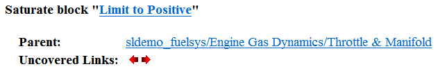
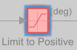
下图显示了 sldemo_fuelsys 示例模型中发动机气体动力学子系统的节气门和歧管子系统中饱和模块的决策分析表。
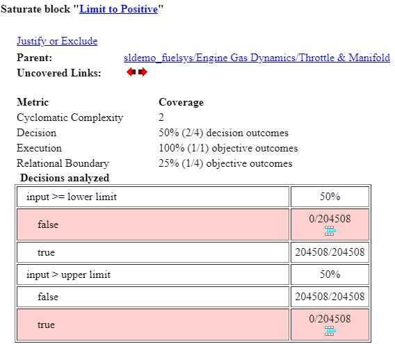
要显示并突出显示有问题的模块,点击包含该模块的决策分析表的部分顶部的模块名称。
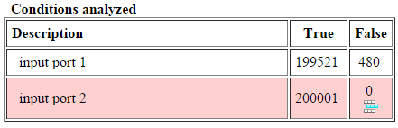
条件分析
分析条件表列出了相应模块的每个输入端口上 true 条件和 false 条件发生的次数。
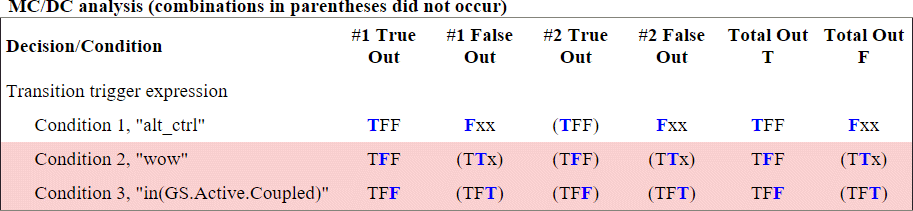
MC/DC 分析
MCDC 分析表列出了相应模块代表的 MCDC 输入条件 case,以及报告的测试用例对这些条件 case 的覆盖程度。
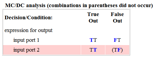
MCDC 分析表的每一行代表针对该模块的特定输入的条件 case。模块的输入 n 的条件 case 是输入值的组合。输入 n 被称为条件 case 的判定输入。单独改变输入 n 的值会改变模块的输出值。
MCDC 分析表以条件 case 表达式来表示一个条件 case。条件 case 表达式是一个字符串,其中:
字符串中字符的位置与输入端口号相对应。
该位置的字符代表输入的值。(
T表示true;F表示false)。粗体字符对应于决策输入的值。
例如,FTF 表示三输入模块的条件 case,其中第二个输入是决策输入。
决策/条件列指定输入条件 case 的决策输入。输出 True 列指定决策输入值,该值导致模块针对条件 case 输出 true 值。输出 True 条目使用条件 case 表达式(例如 FF)来表达模块的所有输入的值,其中决策变量的值以粗体显示。
表达式周围的括号表示指定的输入组合没有在本报告中包含的第一个(或唯一)测试用例中出现。也就是说,该测试用例没有覆盖到相应的条件 case。输出 False 列指定导致模块输出 false 值的决策性输入值,以及该值是否在报告中包含的第一个(或唯一)测试用例期间实际出现。
根据分析期间使用的 MCDC 定义,某些模型元素实现的 MCDC 覆盖率较低。有关分析过程中使用的 MCDC 定义如何影响覆盖率结果的更多信息,请参阅Simulink Coverage 中的修改条件和决策覆盖率 (MCDC) 定义。
如果在配置参数对话框的覆盖率窗格中选择将 Simulink 逻辑模块视为短路,MCDC 覆盖率分析不会验证短路输入是否实际发生。MCDC 分析表使用条件表达式中的 x(例如,TFxxx)来指示工具未经分析的短路输入。
如果禁用此功能,并且在收集模型覆盖率时逻辑模块没有短路,则可能无法实现该模块的 100% 覆盖率。
选择将 Simulink 逻辑模块视为短路选项,以便 MCDC 覆盖率分析可以近似计算测试用例对生成的代码所达到的覆盖率程度(大多数高级语言短路逻辑表达式)。
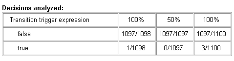
累计覆盖率
记录连续的覆盖率结果后,您可以在覆盖率结果浏览器中进行访问、管理和聚合覆盖率结果。默认情况下,每次仿真的结果都会保存并累积记录在报告中。
如果在配置参数的结果部分中选择显示累积进度报告,累计覆盖率报告所有表最右侧区域的结果将反映运行总值。该报告的组织方式使您可以轻松地将最近运行的附加覆盖率与会话中所有先前运行的覆盖率进行比较。
累计覆盖率报告包含以下信息:
当前运行 - 刚刚完成的仿真的覆盖率结果。
Delta - 刚刚完成的仿真所实现的累积覆盖率中添加的覆盖率百分比。如果前一次仿真的累计覆盖率和当前覆盖率非零,则如果新覆盖率未添加到累计覆盖率中,则增量可能是 0。
累计 - 截至刚刚完成的仿真为止,模型收集的总覆盖率。
运行三个测试用例之后,摘要报告显示第三个测试用例实现的额外覆盖率以及前两个测试用例实现的累计覆盖率。
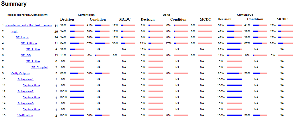
累计覆盖率的分析的决策表包含三列关于决策结果的数据,分别代表当前运行、自上次运行以来的增量和累积数据。
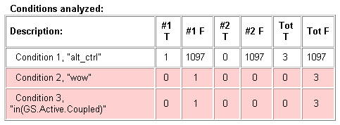
条件分析表使用列标题#n T 和#n F 来指示当前运行和增量的结果。该表使用 Tot T 和 Tot F 表示累积结果。您可以识别每个测试用例相应模块的每个输入端口上的 true 和 false 条件。
MCDC 分析 #n 输出 True 和 #n 输出 False 列显示当前运行和增量的条件 case。T 输出合计和 F 输出合计列显示累积结果。
注意
您可以在命令行计算可重用子系统和 Stateflow 构造的累计覆盖率。有关详细信息,请参阅获取可重用子系统的累积覆盖率。
N 维查找表
下面的交互式图总结了查找表元素的访问程度。在此示例中,两个 Sine Wave 模块生成 x 和 y 索引,用于访问用随机值填充的 10×10 元素的 2-D Lookup Table 模块。
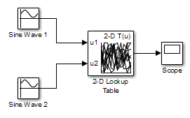
在该模型中,每个方向的查找表索引为 1、2、...、10。正弦波 2 模块与正弦波 1 模块的相位差为 pi/2 弧度。这会为圆的边缘生成 x 和 y 数字,当您检查生成的查找表覆盖率时您会看到这些数字。
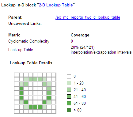
该报告包含一个表示查找表元素的二维表。元素索引由单元格边框网格线表示,每维数字为 10。查找表在表值之间进行插值的区域由单元格区域表示。元素 1 左侧和元素 10 右侧的外推区域由表格边缘的单元格表示,这些单元格没有外边框。
注意
覆盖率报告仅为具有 400 个或更少插值或外推间隔的查找表生成查找表详细信息图像。
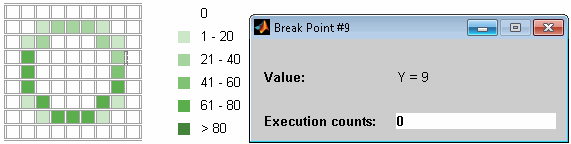
测试期间每个单元格插入或推断的值的数量(执行计数)由分配给该单元格的绿色阴影表示。表格的一侧显示了六个级别的绿色阴影以及所代表的执行计数范围。
如果点击单个表格单元格,您将看到一个对话框,其中显示该单元格的索引位置以及测试期间为其生成的执行计数的确切数量。下面的示例显示了圆圈右边缘上彩色阴影单元格的内容。
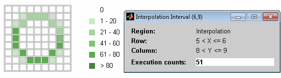
选定的单元格以红色勾勒。您还可以点击表格边缘的外推单元格。
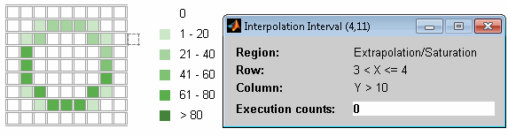
粗体网格线表示在仿真中至少发生一个等于其精确索引值的模块输入。点击边框即可显示该索引值的精确命中次数。
以下示例模型使用一个由随机值填充的 10×10×5 元素组成的 n-D Lookup Table 模块。
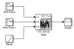
X 和 y 表轴的索引均为 1、2、...、10。Z 轴的索引为 10、20、...、50。在上面的示例中,使用两个 Sine Wave 模块生成的 x 和 y 索引以及 Ramp 模块生成的 z 索引来访问查找表值。
仿真之后,您会看到以下查找表报告。
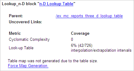
链接 Force Map Generation 不是显示二维表,而是显示以下表:
三维查找表模块的查找表覆盖率被报告为一组二维表。
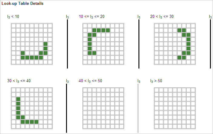
垂直条代表精确的 z 索引值:10、20、30、40、50。如果垂直条为粗体,则表示至少有一个模块输入等于它在仿真期间所代表的精确索引值。点击某个条形图即可获得该条形图所代表的精确索引值的覆盖率报告。
您可以报告任意维度的查找表的查找表覆盖率。四维表的覆盖率被报告为三维集的集合,就像前面示例中的集合一样。五维表被报告为三维集的集合,依此类推。
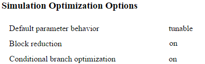
模块简化
所有模型覆盖率报告都会在报告开头指明 Simulink 模块简化参数的状态。在以下示例中,您设置了强制关闭模块简化。
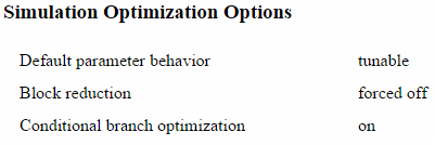
在下一个示例中,您启用了 Simulink 模块简化参数,但未设置强制关闭模块简化。
考虑以下模型,其中仿真不执行 MinMax1 模块,因为只有一个输入 - In3。
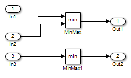
如果设置了强制关闭模块简化,则报告不包含此模块的覆盖率数据,因为 MinMax1 模块的最小输入始终是 1。
如果不设置强制关闭模块简化,报告则不包含减少模块的覆盖率数据。
关系边界
在配置参数对话框的 覆盖率窗格 上,如果选择关系边界覆盖率度量,软件会在模型覆盖率报告中为支持此覆盖率的每个模型对象创建一个关系边界表。该表适用于模型对象所涉及的显式或隐式的关系操作。有关详细信息,请参阅:
接受覆盖率的模型对象 中的关系边界列。
下表显示了关系 input1 <= input2 的关系边界覆盖率报告。表的外观取决于操作数的数据类型。
整数
如果两个操作数都是整数(或者一个操作数是整数,另一个是布尔值),则表格如下所示。
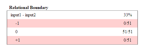
对于关系运算如 operand_1 <= operand_2
第一行以
operand_1-operand_2第二行表示仿真过程中
operand_1-operand_2第三行表示仿真过程中
operand_1operand_2第四行表示仿真过程中
operand_1-operand_2
定点
如果其中一个操作数具有定点类型,而另一个操作数是定点或整数,则表格如下所示。LSB 表示最低有效位的值。有关详细信息,请参阅精度 (Fixed-Point Designer)。如果两个操作数的精度不同,则使用较小的精度值。
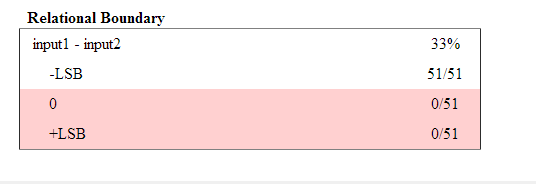
对于关系运算如 operand_1 <= operand_2
第一行以
operand_1-operand_2第二行表示仿真过程中
operand_1-operand_2-LSB的次数。第三行表示仿真过程中
operand_1operand_2第四行表示仿真过程中
operand_1-operand_2LSB的次数。
浮点
如果其中一个操作数具有浮点类型,则表格如下所示。tol 表示使用输入值和您指定的容差计算的值。如果您未指定容差,则使用默认值。有关详细信息,请参阅关系边界覆盖率。
![Relational Boundary coverage table: Row 1 displays input1 - input 2: 50% coverage. Row 2 displays [-tol.. 0]: 51/51. Row 3 displays (0..tol]: 0/51.](coverage_relational_boundary.png)
对于关系运算如 operand_1 <= operand_2
第一行以
operand_1-operand_2第二行显示了仿真过程中
operand_1-operand_2[-tol..0]范围内的次数。第三行显示了在仿真仿真中
operand_1-operand_2(0..tol]范围内的次数。
该表的外观根据模块中的关系运算符而变化。根据关系运算符,operand_1 - operand_2
排除在关系边界覆盖率之外。
包含在关系边界之上的区域内。
包含在关系边界以下的区域内。
| Relational Operator | 报告格式 | 说明 |
|---|---|---|
== | [-tol..0) | 0 被排除。 |
(0..tol] | ||
!= | [-tol..0) | 0 被排除。 |
(0..tol] | ||
<= | [-tol..0] | 0 包含在关系边界以下的区域中。 |
(0..tol] | ||
< | [-tol..0) | 0 包含在关系边界上方的区域中。 |
[0..tol] | ||
>= | [-tol..0) | 0 包含在关系边界上方的区域中。 |
[0..tol] | ||
> | [-tol..0] | 0 包含在关系边界以下的区域中。 |
(0..tol] |
0 包含在 <= 的关系边界之下,但包含在 < 的关系边界之上。该规则与决策覆盖率一致。例如:
对于关系
input1 <= input2,如果input1小于或等于input2,则判定为 true。<和=被分组在一起。因此,0 位于关系边界以下的区域。对于关系
input1 < input2,仅当input1小于input2时,判定才为 true。>和=被组合在一起。因此,0 位于关系边界上方的区域。
整数溢出分析
在配置参数对话框的 覆盖率窗格 上,如果选择对整数溢出进行饱和处理覆盖率度量,软件会在模型覆盖率报告中创建一个溢出饱和度分析表。该软件为选择了对整数溢出进行饱和处理参数的每个模块创建表。
溢出饱和分析表列出了模块在整数溢出时饱和的次数,表示做出正确的决策。如果模块在整数溢出时没有饱和,则该表指示 false 决策。未发生的结果以红色突出显示的表行表示。
下图显示了 sldemo_fuelsys 示例模型中发动机气体动力学子系统的混合与燃烧子系统中 MinMax 模块的溢流饱和度分析表。
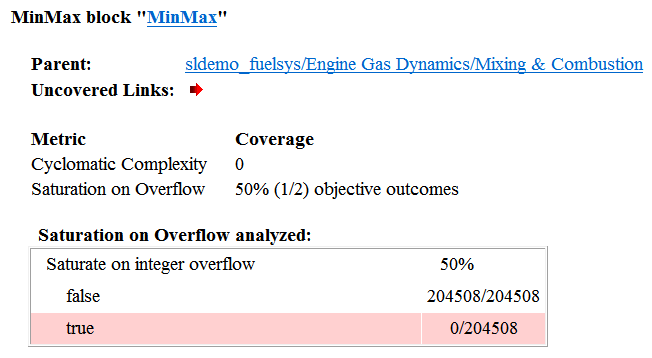
要显示并突出显示有问题的模块,点击包含该模块的溢出饱和度分析表的部分顶部的模块名称。

信号范围分析
如果您选择信号范围覆盖率度量,软件会在模型覆盖率报告的底部创建一个信号范围分析部分。本节列出了仿真过程中测得的模型中每个输出信号的最大和最小信号值。
使用模型覆盖率报告顶部非滚动区域中的信号范围链接快速访问信号范围分析报告,如下面的 sldemo_fuelsys 示例模型报告所示。
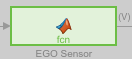
每个模块都以分层方式报告;子模块直接出现在父模块之下。信号范围报告中的每个模块名称都是一个链接。例如,选择 EGO sensor 链接以在其原生图中突出显示此模块。
可变维度信号的信号尺寸覆盖率
如果选择信号大小,软件会在模型覆盖率报告中的信号范围数据后创建一个可变信号宽度部分。本节列出了模型中具有可变大小信号的所有输出端口的最大和最小信号大小。它还列出了 Simulink 为该信号分配的内存,如在仿真期间测量的。此列表不包括在仿真中大小不会变化的信号。
以下示例显示了覆盖率报告中的可变信号宽度部分。在此示例中,Abs 模块信号大小从 2 变化到 5,分配为 5。
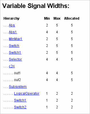
每个模块都以分层方式报告;子模块直接出现在父模块之下。可变信号宽度列表中的每个模块名称都是一个链接。点击链接会突出显示 Simulink 编辑器中的相应模块。经过分析,可变尺寸的信号具有更宽的线路设计。
Simulink Design Verifier 覆盖率
如果您选择目标和约束,分析将收集模型中所有 Simulink Design Verifier 模块的覆盖率数据。
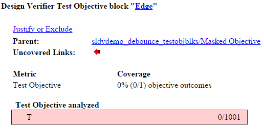
要了解其工作原理,请打开 sldvdemo_debounce_testobjblks 模型。
该模型包含两个 Test Objective 模块:
True 模块定义了一个属性,即信号具有
2的值。Masked Objective 子系统内的 Edge 模块描述了 Masked Objective 子系统中 AND 模块的输出从
2变为1的属性。
Simulink Design Verifier 软件分析该模型并生成包含实现特定测试目标的测试用例的框架模型。要查看原始模型是否实现了这些目标,仿真框架模型并收集模型覆盖率数据。模型覆盖率工具分析您在 Test Objective 模块中指定的区间内的任何决策点或值。
在此示例中,覆盖率报告显示您实现了 True 模块的 100% 覆盖率,因为信号值至少出现一次 2。在 14 个时间步中,有 6 个时间步的信号值为 2。
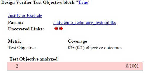
Edge 模块的输入信号在 14 个时间步中达到一次 True 的值。