Estimate Vehicle Drag Coefficients by Coast-Down Testing

Since R2023b

This example uses:

This example shows how to estimate the drag coefficients of a vehicle using parameter estimation with data obtained from coast-down testing. Coast-down testing of a vehicle is performed by running the vehicle at a constant speed before letting it coast down at idle throttle and measuring the vehicle velocity over time. The velocity decays due to several sources of drag, including fixed resistances, drivetrain and rolling resistances, and aerodynamic drag resistance. Drivetrain and rolling resistances scale with the velocity, while aerodynamic resistance scales with the square of velocity. Thus, fitting the drag force to a polynomial of the form $F_{drag} = a + b \dot{x} + c {\dot{x}}^{2}$ lets you estimate the coefficients for each type of drag. This coast-down testing procedure is specified in SAE standard J1263.

Coast-Down Model

The Simulink® model coastdownmodel.slx uses the block Vehicle Body Total Road Load (Vehicle Dynamics Blockset). Open the model.

mdl = "coastdownmodel";
open_system(mdl)

Coast-Down model

The Vehicle Body Total Road Load block implements the dynamic coast-down model $F_{drag} = a + b \dot{x} + c {\dot{x}}^{2}$ , where:

Cd = c is the aerodynamic drag coefficient.
Cr = b is the coefficient for drivetrain and rolling resistance.
Cr0 = a is the coefficient for the fixed resistances.

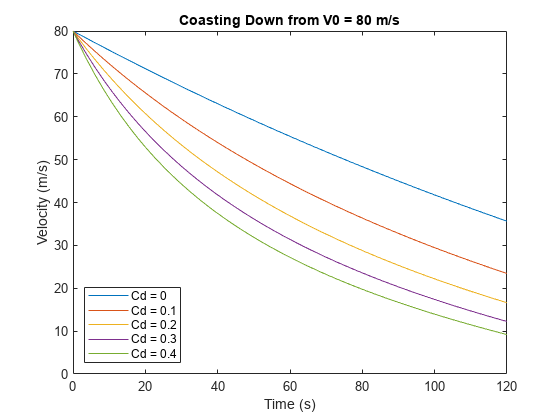
To illustrate the effects of the drag coefficients, try simulating the model with varying Cd, fixing the values of the other two coefficients and assuming the vehicle mass is 1800 kg. Plot the velocity versus time for Cd values ranging from 0 to 0.4 in 0.1 increments and an initial velocity of 80 m/s. The plot shows that higher aerodynamic drag coefficients lead to much more deceleration and thus a faster coast-down curve.

Cd_vec = 0.0:0.1:0.4;
Cr = 6.5;   % drivetrain/rolling resistance
Cr0 = 300;  % fixed resistances
M = 1800;   % vehicle mass
V0 = 80;    % initial velocity

for Cd = Cd_vec
    out = sim("coastdownmodel.slx");
    t = out.tout;
    xdot = out.yout(:,2);
    plot(t,xdot,"DisplayName","Cd = " + string(Cd));
    hold on
end

xlabel("Time (s)")
ylabel("Velocity (m/s)")
xlim([0 120])
legend("Location","southwest")
title("Coasting Down from V0 = 80 m/s")
hold off

Figure contains an axes object. The axes object with title Coasting Down from V0 = 80 m/s, xlabel Time (s), ylabel Velocity (m/s) contains 5 objects of type line. These objects represent Cd = 0, Cd = 0.1, Cd = 0.2, Cd = 0.3, Cd = 0.4.

Measured Data

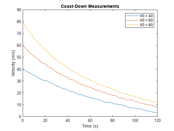
If you have measured coast-down data, you can use the Parameter Estimator app with this model to estimate the coefficients of the vehicle used for the measurement. For this example, load coast-down data obtained using initial velocities V0 = 40, 60, and 80 m/s. The data is stored in the structure measData.

load coastDownExampleData.mat measData
measData

measData = struct with fields:
       t_40: [59x1 double]
    xdot_40: [59x1 double]
       t_60: [60x1 double]
    xdot_60: [60x1 double]
       t_80: [60x1 double]
    xdot_80: [60x1 double]

plot(measData.t_40,measData.xdot_40,...
    measData.t_60,measData.xdot_60,...
    measData.t_80,measData.xdot_80)
legend("V0 = 40","V0 = 60","V0 = 80")
xlabel("Time (s)")
ylabel("Velocity (m/s)")
title("Coast-Down Measurements")

Figure contains an axes object. The axes object with title Coast-Down Measurements, xlabel Time (s), ylabel Velocity (m/s) contains 3 objects of type line. These objects represent V0 = 40, V0 = 60, V0 = 80.

Parameter Estimation with Data

To use the measured data for parameter estimation, open the Parameter Estimator app for coastdownmodel by clicking Parameter Estimator in the Apps tab of the model. In the app, create a new experiment for the V0 = 40 data. Under Output Signals, for the xdot output signal of the Vehicle Body Total Road Load block, set the measured data to [measData.t_40,measData.xdot_40].

Then, under Initial States, select the model state coastdownmodel/Vehicle Body Total Road Load/Vehicle Body Total Road Load Power Input/Integrator2. This state feeds the xdot output and corresponds to the velocity of the vehicle. Therefore, set its initial value to 40, and clear the Estimate checkbox for this state.

The following screenshot shows the Edit Experiment dialog box for this V0 = 40 data.

Edit Experiment: Exp_40 dialog box with Outputs and Initial State sections filled in as mentioned

Click Plot to create an experiment plot in the app, and click Close to save the experiment.

Next, return to the Parameter Estimation tab and create similar experiments and experiment plots for the V0 = 60 and V0 = 80 coast-down data. For more details about how to configure experiment data and initial states for parameter estimation, see Specify Estimation Data and Specify Known Initial States.

Specify Parameters to Estimate

Next, select and configure the parameters to estimate. In the app, click Select Parameters. In the Edit: Estimated Parameters dialog box, click Select Parameters. Then specify the model parameters Cd, Cr, and Cr0 as continuous-valued parameters for estimation.

Select model variables dialog box with Cd, Cr, and Cr0 selected as Continuous variables

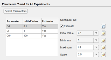
Set the minimum allowed value of all three parameters to zero to ensure that the estimated values are positive. Set the initial values as follows:

Cd — 0.1
Cr — 1
Cr0 — 100

The app uses these values as initial guesses for the estimation.

Parameters Tuned for All Experiments section showing Cd, Cr, and Cr0 with their initial values

For more details on configuring parameters for estimation, see Specify Parameters for Estimation.

Estimate Parameters

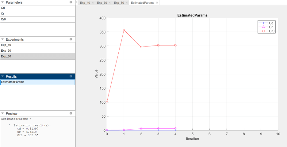
To begin the estimation, click Estimate. The app estimates the parameter values by repeatedly simulating the model and evaluating the default cost function. The estimation process looks for parameter values that minimize the cost function. For this problem, the estimation takes only a few iterations to converge.

Parameter trajectory plot

To view the estimated parameter values, under Results, select EstimatedParams. The resulting estimated values of the three drag coefficients are shown under Preview.

Cd — 0.31397
Cr — 6.4219
Cr0 — 302.5

The app updates the experiment plots to compare the measured data against the results of simulating the model at each initial velocity with these estimated parameter values.

Amplitude vs Time plots for Exp_40, Exp_60, and Exp_80

The plots show that simulating the model at V0 = 40, V0 = 60, and V0 = 80 using these parameter values results in coast-down curves that closely match the measured velocity curves. You can further validate the estimated parameter values using coast-down data measured independently from the data used for estimation (see Validate Estimation Results).