Specifying Variable Inertias
Modeling Variable Inertias
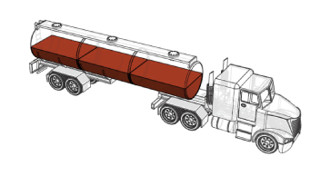
A variable inertia is a mass element whose mass, center of mass, or inertia tensor can vary through time. Variable inertias include the scooped contents of a backhoe bucket, the moving occupants of a boom manlift, and the sloshing fluid load of a decelerating tank truck. You model a variable inertia using the General Variable Mass block from the Body Elements > Variable Mass library. This block accepts the various inertial properties as constants or variables. Physical signal ports provide the means to specify the variable properties.
A Fluid Load as a Variable Inertia

Specifying the Variable Inputs
You can specify your variable inputs using Simscape™ or Simulink® blocks. You must convert any Simulink signals into physical signals using the Simulink-PS Converter block. Avoid sudden changes as these can increase model stiffness and slow down simulation. Ensure that the signal dimensions agree with the ports:
Scalar for mass (port m)
Three-element vector for center of mass (port com)
Nine-element matrix for inertia tensor (port I)
Visualizing Variable Inertias
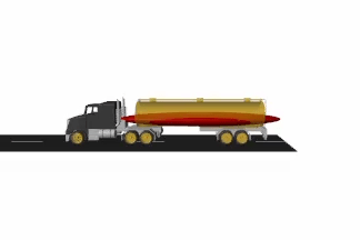
Variable inertias associated with General Variable Mass blocks have no geometry. You must visualize these inertias as graphical markers or as equivalent inertia ellipsoids. The ellipsoid dimensions and geometry center vary with mass, center of mass, and inertia tensor, lending the ellipsoids to more informative model visualizations. Inertia markers are shown on model update and during simulation. Variable inertia ellipsoids are shown during simulation only. The figure shows an inertia visualization representing a fluid load carried by a tank truck.
Equivalent Inertia Ellipsoid Visualization

Modeling Body Interactions
The General Variable Mass block captures inertial effects only. Any interactions between variable inertias and other model components must be modeled explicitly. Examples of interactions include contact forces between the fluid load of a tank truck and the surrounding enclosure. They include also the change in momentum obtained by expelling the combustion products of a propulsion system—for example, in a marine or space vehicle. Use other Simscape Multibody™, Simscape, and Simulink blocks to capture interactions like these.
Model a Variable-Mass Oscillator
Create a simple model of a mass-spring system to simulate under constant-mass and variable-mass conditions. The model uses a General Variable Mass block to represent a container onto which a load of sand is progressively dropped. A Cartesian Joint block provides the variable-mass body with three translational degrees of freedom, although only one—along the vertical z-axis—is relevant during simulation. A Spring and Damper Force block represents the spring element, which connects the variable-mass body to the World frame.

Create Block Diagram
At the MATLAB® command prompt, enter
smnew. The command opens a model template with commonly used Simscape Multibody blocks.Add the following blocks to the model canvas:
General Variable Mass (Body Elements > Variable Mass)
Cartesian Joint (Joints)
Spring and Damper Force (Forces and Torques)
Connect the blocks as shown in the figure and delete the remaining blocks. Ensure that the joint block orientation is as shown, with the base frame port facing the World Frame block.

In the Spring and Damper Force block dialog box, set the Natural Length parameter to
0.2m and the Spring Stiffness parameter to10N/m.In the Cartesian Joint block dialog box, expand the Z Prismatic Primitive (Pz) area, select the State Targets > Specify Position Target check box, and set the Value parameter to
0.1m.
Add Position Sensing
In the Cartesian Joint block dialog box, expand the Z Prismatic Primitive (Pz) area and select the Sensing > Position check box. The block exposes a physical signal output port with the oscillator frame position.
Add the following blocks to the model canvas:
PS-Simulink Converter (Simscape > Foundation Library > Utilities)
Scope (Simulink > Sinks)
Connect the blocks as shown in the figure.

Simulate with Constant Mass
In the General Variable Mass block dialog box, set the Type parameter to
Custom. This option enables you to model a variable mass distribution with rotational inertia.Set the Mass, Center of Mass, and Inertia Matrix parameters to
Constantand the Mass > Value parameter to0.2kg.Run the simulation and open the Scope block. The plot shows the position of the reference frame of the variable mass. Note that the oscillation frequency and amplitude stay constant throughout simulation.

Multibody Explorer opens with a 3-D animation of the model. The visualization comprises only an inertia ellipsoid—here a sphere due to the symmetry of the default inertia tensor used in the model. In the menu bar, select View > Show Frames to show all the frames in the model. Note that the ellipsoid dimensions stay constant during simulation, reflecting the constant inertial properties specified in the model.

Simulate with Variable Mass
In the General Variable Mass block dialog box, set the Center of Mass and Inertia Matrix parameters each to
Constant. The physical signal ports used to vary their values during simulation become hidden, leaving only the solid mass as a variable.Add these blocks to the model canvas:
Simulink-PS Converter (Simscape > Foundation Library > Utilities)
Ramp (Simulink > Sources)
Connect the blocks as shown in the figure.

In the Ramp block dialog box, set the Slope parameter to
0.1and the Initial output parameter to0.2. The Ramp signal is passed to the General Variable Mass block in the default Simscape units of mass, kg. The signal corresponds to a steadily increasing mass that starts at0.2kg and ends at1.2kg following a 10-second simulation.Run the simulation and open the Scope block. The position plot shows a variable oscillation frequency and amplitude. The increasing mass causes the oscillation frequency to increase and the amplitude to decrease.

Multibody Explorer updates the visualization results. Note that the ellipsoid dimensions decrease as the simulation progresses, reflecting their inverse proportionality to the variable mass.
