Running a Grid-Connected PV Array Model in Real-Time Using Decoupling Line Blocks

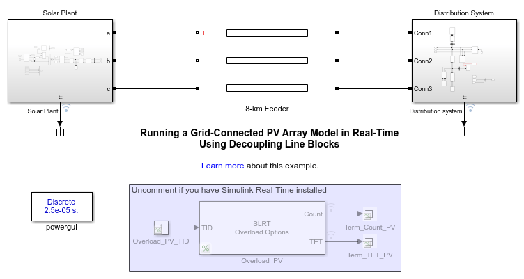
1. The Base Model

As a base model, use a simplified version of the Running a Grid-Connected PV Array Model in Real-Time Using Decoupling Line Blocks example. This base example is available in the DecoupledPVArrayGrid.slx file:

model='DecoupledPVArrayGrid';
open_system(model);

Simulate the model and observe simulation signals using the Simulink Data Inspector.

Three events are programmed in the simulation: an irradiance variation, a reactive power reference step, and a two-phase fault on the distribution system:

2. Run the Base Model in Real-Time

This code is a summary of the settings made to the base model to run in real-time.

First enable data logging for the number of overload count and the Task Execution Time (TET):

set_param([model,'/Overload_PV'],'TETFlag','on');
set_param([model,'/Overload_PV'],'StartupDur','1000');
set_param([model,'/Overload_PV'],'maxOverload','100000');

ph = get_param([model,'/Overload_PV'],'PortHandles');
set_param(ph.Outport(1),'DataLogging','on');
set_param(ph.Outport(1),'DataLoggingNameMode','Custom');
set_param(ph.Outport(1),'DataLoggingName','Overload_Count_PV');

ph = get_param([model,'/Overload_PV'],'PortHandles');
set_param(ph.Outport(2),'DataLogging','on');
set_param(ph.Outport(2),'DataLoggingNameMode','Custom');
set_param(ph.Outport(2),'DataLoggingName','Overload_TET_PV');

Then prepare the model for code generation using speedgoat.tlc as system target file:

cs = getActiveConfigSet(model);
switchTarget(cs,'speedgoat.tlc',[]);
set_param(model,'SolverType','Fixed-step');
set_param(model,'SolverName','FixedStepDiscrete');
set_param(model,'GenCodeOnly', 'off');
set_param(model,'MaxIdLength', 95);

Now, assuming you have a Speedgoat target machine hardwired to your host computer, connect, build, load, and run the model on the target with these commands:

tg=slrealtime;
connect(tg);
slbuild(model);
load(tg,model);
pause(5);
tg.start;

Using the Data Inspector, see that the average execution time exceeds the model sample time (2.5e-5sec), producing a large amount of overloads that prevent the model to accurately run in real-time.

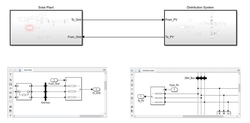
3. Split the Base Model with Decoupling Line Blocks

To avoid CPU overloads in real-time, two Decoupling Line blocks can be used to split the model into two separate tasks that can run concurrently on the Speedgoat multi-core target.

You can use the Line Decoupler App to replace the Distributed Parameter Line block, that connects the solar plant to the distribution system, with a pair of Decoupling Line blocks. Access the App from the command line:

DecouplingLineReplace(model)

The App lists all the Distributed Parameters Line blocks in the model. Select the 8-km Feeder block in the list, and click Replace. The block is automatically replaced by a pair of Decoupling Line blocks that are tuned with the parameters of the original Distributed Parameter Line block.

Now that there are no more electrical connections between the two ends of the line, move the 8-km Feeder Send block inside the Solar Plant subsystem, and move the 8-km Feeder Receiving block inside the Distribution System subsystem. Move the powergui block and the Overload_PV blocks into the Solar Plant subsystem and make a copy of both blocks into the Distribution System.

In the Solar Plant subsystem, check the Show send and receiving ports parameter of the Decoupling Line block. This option replace the internal Goto and From blocks with Inport r and Outport s blocks. This allow us to connect an Inport block and an Outport to the block. Remove the measurement output port. In the Distribution System, apply the same modifications. Finally, connect the two subsystems together:

4. Prepare the Decoupled Model for Concurrent Execution

The code below is a summary of the settings you need to make to the model to run it in real-time on a Speedgoat target:

Simulink.architecture.config(model, 'Convert');
Simulink.architecture.importAndSelect(model,'Multicore');
Simulink.architecture.get_param(model,'ArchitectureName');
set_param(model,'ExplicitPartitioning','on');

for i=1:2
  Simulink.architecture.add('Task', [model, '/CPU/Periodic/Task', num2str(i)]);
  Simulink.architecture.set_param([model, '/CPU/Periodic/Task',num2str(i)], 'Period', 'Ts');
end

dt = get_param(model, 'DataTransfer');
dt.DefaultTransitionBetweenSyncTasks = 'Ensure deterministic transfer (maximum delay)';

for i=1:2
  set_param([model, Subsystems{i}],'TargetArchitectureMapping', [model, '/CPU/Periodic/Task',num2str(i)]);
end

5. Build, Load, and Run the Decoupled Model on the Target

Now, assuming that your host computer is connected to your Speedgoat target you can build, load, and run the decoupled model in real-time:

slbuild(model)

tg=slrealtime;
load(tg,model)
pause(5)

tg.start

The next figure shows simulation signals in the Data Inspector. See that the average execution time no longer exceeds the model sample time (subplot on the bottom left).

By using the Decoupling Line block and a multicore target, you can run the model in real-time without CPU overload.