使用 Stateflow API 创建图
R2026b此示例说明如何使用 Stateflow 应用程序编程接口 (API) 创建一个 Stateflow® 图。Stateflow API 是一个通过 MATLAB® 命令创建或更改 Stateflow 图的工具。有关详细信息,请参阅Stateflow API 概述。
创建 Stateflow 图
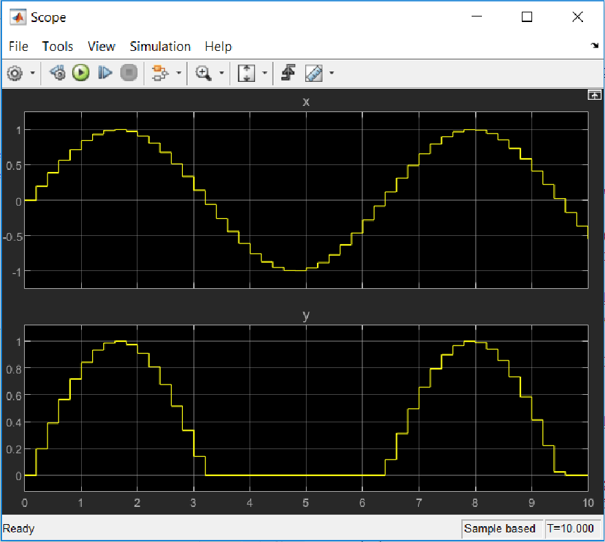
此 Stateflow 图展示半波整流器的基础逻辑。该图包含两个标签为 On 和 Off 的状态。在 On 状态下,图输出信号 y 等于输入 x。在 Off 状态下,输出信号设置为零。当输入信号跨越某个阈值 t0 时,图在这些状态之间转移。各个状态下的动作在仿真的每一时间步都会更新 y 的值。
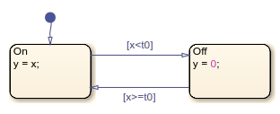
有关仿真此图的详细信息,请参阅创建 Stateflow 图。
1.创建一个名为 rectify 的 Simulink® 模型,其中包含一个空的 Stateflow Chart 模块。
sfnew rectify2.通过调用 find 函数访问模型中与图对应的 Stateflow.Chart 对象。使用函数 sfroot 访问 Simulink.Root 对象,它是 Stateflow API 中所有对象的父级。
ch = find(sfroot,"-isa","Stateflow.Chart", ...
    Path="rectify/Chart");
3.通过调用 view 函数在 Stateflow 编辑器中打开图。
view(ch);
4.通过修改图的 ActionLanguage 属性更改动作语言。
ch.ActionLanguage = "C";添加状态
要将 Stateflow API 对象创建为父对象的子对象,请将父对象用作创建子对象的函数的输入参量。有关详细信息,请参阅Create and Delete Stateflow Objects。
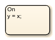
1.调用 Stateflow.State 函数以向图添加状态。
s1 = Stateflow.State(ch);
2.通过更改对应 State 对象的 Position 属性调整状态的位置。将新位置指定为一个四元素向量,其中前两个值是状态左上角的 (x,y) 坐标,后两个值是状态的宽度和高度。
s1.Position = [30 30 90 60];
3.通过更改 LabelString 属性指定状态的名称和标签,如Specify Labels in States and Transitions Programmatically中所述。
s1.LabelString = "On"+newline+"y = x;";
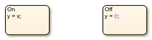
4.创建第二个状态。调整其位置并指定其名称和标签。
s2 = Stateflow.State(ch);
s2.Position = [230 30 90 60];
s2.LabelString = "Off"+newline+"y = 0;";
添加转移
当添加转移时,通过修改其 Source 和 Destination 属性指定其源和目标。对于默认转移,您指定目标,但不指定源。
1.调用 Stateflow.Transition 函数以向图添加转移。
t1 = Stateflow.Transition(ch);
2.设置转移源和目标。
t1.Source = s1;
t1.Destination = s2;
3.通过修改其 SourceOClock 属性调整转移的位置。
t1.SourceOClock = 2.1;
4.通过更改 LabelString 和 LabelPosition 属性指定转移标签及其位置。
t1.LabelString = "[x<t0]";
t1.LabelPosition= [159 23 31 16];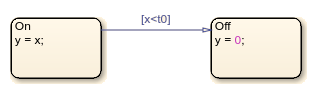
5.创建第二个转移。指定其源、目标和标签。
t2 = Stateflow.Transition(ch);
t2.Source = s2;
t2.Destination = s1;
t2.SourceOClock = 8.1;
t2.LabelString = "[x>=t0]";
t2.LabelPosition= [155 81 38 16];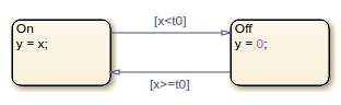
6.添加到状态 On 的默认转移。要创建垂直转移,请修改 SourceEndpoint 和 Midpoint 属性的值。有关详细信息,请参阅添加默认转移。
t0 = Stateflow.Transition(ch);
t0.Destination = s1;
t0.DestinationOClock = 0;
t0.SourceEndpoint = t0.DestinationEndpoint-[0 30];
t0.Midpoint = t0.DestinationEndpoint-[0 15];
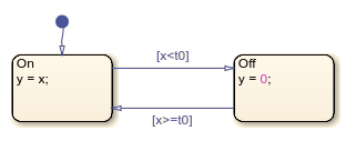
添加数据
必须定义图中使用的每个数据符号并指定其作用域和类型,才能对图进行仿真。
1.调用 Stateflow.Data 函数以添加表示图输入的数据对象。
x = Stateflow.Data(ch);
2.将数据对象的名称指定为 x,并将其作用域指定为 Input。
x.Name = "x";
x.Scope = "Input";
3.要指定输入 x 具有类型 double,请将其 Props.Type.Method 属性设置为 Built-in。默认内置数据类型为 double。
x.Props.Type.Method = "Built-in";
x.DataType
ans = 'double'
4.添加表示图输出的数据对象。将其名称指定为 y,并将其作用域指定为 Output。
y = Stateflow.Data(ch);
y.Name = "y";
y.Scope = "Output";
5.要指定输出 y 具有类型 single,请将其 Props.Type.Method 属性设置为 Built-in,并将其 DataType 属性设置为 single。
y.Props.Type.Method = "Built-in";
y.DataType = "single";
y.DataType
ans =
'single'
6.添加表示图中转移阈值的数据对象。将其名称指定为 t0,并将其作用域指定为 Constant。将其初始值设置为 0。
t0 = Stateflow.Data(ch);
t0.Name = "t0";
t0.Scope = "Constant";
t0.Props.InitialValue = "0";
7.要指定阈值 t0 具有定点数据类型,请将其 Props.Type.Method 属性设置为 Fixed-point。然后指定应用于定点数据的 Props.Type 属性的值。
t0.Props.Type.Method = "Fixed point";
t0.Props.Type.Signed = true;
t0.Props.Type.WordLength = "5";
t0.Props.Type.Fixpt.ScalingMode = "Binary point";
t0.Props.Type.Fixpt.FractionLength = "2";
t0.DataType
ans =
'fixdt(1,5,2)'
保存和仿真图
要保存包含已完成图的模型,请调用 sfsave 函数。
sfsave
要仿真图,请通过输入端口和输出端口将其连接到 Simulink 模型中的其他模块。
1.向模型添加并连接源:
source = add_block("simulink/Sources/Sine Wave","rectify/Sine Wave");
set_param(source, ...
    SampleTime="0.2", ...
    Position=[-105 30 -75 60]);

sourcePorts = get_param(source,"PortConnectivity");
chartPorts = get_param("rectify/Chart","PortConnectivity");

add_line("rectify",[sourcePorts(1).Position; chartPorts(1).Position]);
2.向模型添加并连接信宿:
sink = add_block("simulink/Sinks/Scope","rectify/Scope");
set_param(sink, ...
    NumInputPorts="2", ...
    Position=[185 21 215 54]);

sinkPorts = get_param(sink,"PortConnectivity");

add_line("rectify", [-25 45; -25 -10; 135 -10; 135 30; 180 30]);
add_line("rectify",[chartPorts(2).Position; sinkPorts(2).Position]);
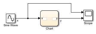
3.对模型进行仿真。
sim("rectify");4.双击 Scope 模块。示波器显示 Stateflow 图的输入信号和输出信号图。