distplot

Plot Survivor Function

Return the survivor function values of the model, evaluated at 50 equally spaced time values between 0.8 and 10. By default, the software calculates the survivor function at the lowest unique stressor level in mdl.StressorLevels. In this example, the lowest unique stressor level corresponds to a humidity value of 50% and a temperature of 5 degrees Celsius.

points = linspace(0.8,10,50)';
x = distfcn(mdl,EvaluationTimes=points)

x = 50×1

    0.8000
    0.9878
    1.1755
    1.3633
    1.5510
    1.7388
    1.9265
    2.1143
    2.3020
    2.4898
    2.6776
    2.8653
    3.0531
    3.2408
    3.4286
      ⋮

Plot the survivor function at the evaluation points.

distplot(mdl,EvaluationTimes=points)

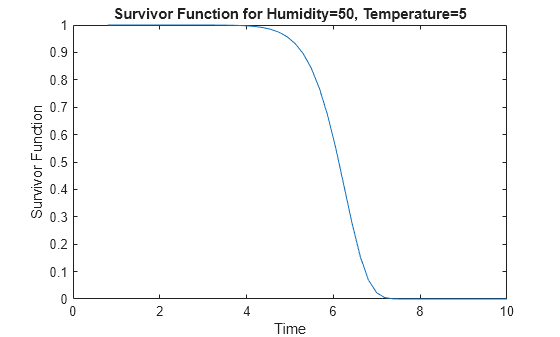
The plot shows that, at this stressor level, the assembly line part has a survival probability close to 100% for time values smaller than 4. The survival probability drops to approximately zero for time values greater than 7.5.

Plot Probability Density Function

Plot the probability density function (pdf).

distplot(mdl,Type="pdf",EvaluationTimes=points)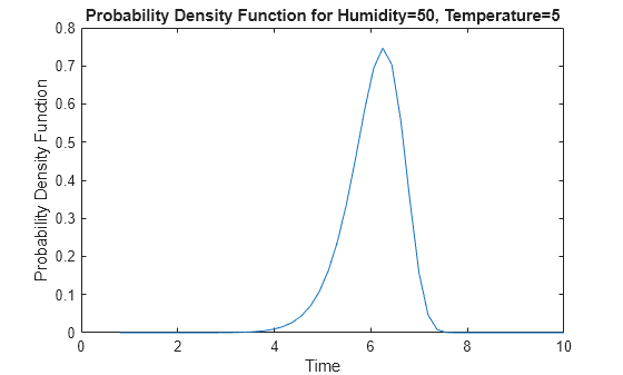

The plot shows that the most likely failure time at this stressor level is approximately 6.2.

Plot Cumulative Distribution Function

Plot the cumulative distribution function (cdf) at a stressor level that corresponds to 90% humidity and a temperature of 20 degrees.

distplot(mdl,[90 20],Type="cdf",EvaluationTimes=points)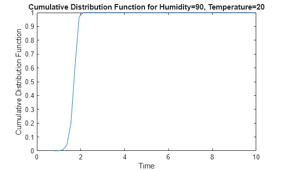

The plot shows that, at this stressor level, approximately half of all assembly line parts have failure times smaller than 1.7.

Plot Inverse Cumulative Distribution Function

Calculate the inverse cumulative distribution function (icdf) at 90% humidity and 35 degrees, and 90% humidity and 20 degrees. Evaluate the icdf at 10 equally spaced probability values between 0.1 and 0.9.

pts = linspace(0.05,0.9,10);
icdfval = [icdf(mdl,pts); icdf(mdl,pts,[90,20])]

icdfval = 2×10

    4.9953    5.4502    5.6944    5.8737    6.0227    6.1562    6.2834    6.4119    6.5525    6.7298
    1.3842    1.5102    1.5779    1.6275    1.6688    1.7058    1.7411    1.7767    1.8156    1.8648

Create a plot of the icdf values for the two stressor levels.

plot(pts,icdfval,"-o")
xlabel("Probability")
ylabel("ICDF Value")
legend(["Humidity = 90, Temperature = 35", ...
    "Humidity = 90, Temperature = 20"],Location="east")

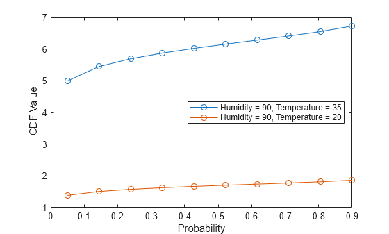
The icdf values are consistently lower at the lower temperature stressor level.