Main Content

ccdesign

Central composite design

Description

dCC = ccdesign(n) returns a numeric matrix dCC containing a central composite (Box-Wilson) design for n factors, where n is a positive integer scalar in the range [2, 26]. The size of dCC is m-by-n, where m is the number of runs (points) in the design. Each row of dCC contains the settings of all factors for that run. The factor values are normalized so that the cube points take values between –1 and 1.

example

dCC = ccdesign(n,Name=Value) returns dCC with additional options specified by one or more name-value arguments. For example, you can specify the number of center points, and the maximum number of points per block.

example

[dCC,blocks] = ccdesign(___) additionally returns a 1-by-m vector containing the block numbers for each run, using any of the input argument combinations in the previous syntaxes. The blocks indicate the runs to measure under similar conditions in order to minimize the effect of inter-block differences on the parameter estimates.

example

Examples

collapse all

Create a two-factor central composite circumscribed design.

dCC = ccdesign(2);

Display the last 10 runs of the design.

disp(dCC(end-9:end,:))
         0   -1.4142
         0    1.4142
         0         0
         0         0
         0         0
         0         0
         0         0
         0         0
         0         0
         0         0

The design contains eight center points to reduce the correlations among the coefficient estimates.

Visualize the design.

plot(dCC(:,1),dCC(:,2),"ro",MarkerFaceColor="b")
X = [1 -1 -1 -1; 1 1 1 -1];
Y = [-1 -1 1 -1; 1 -1 1 1];
line(X,Y,Color="b")
axis square equal

Figure contains an axes object. The axes object contains 5 objects of type line. One or more of the lines displays its values using only markers

The coordinates of each point represent the factor settings of a run in the design. In the circumscribed design, four points are located outside the main square.

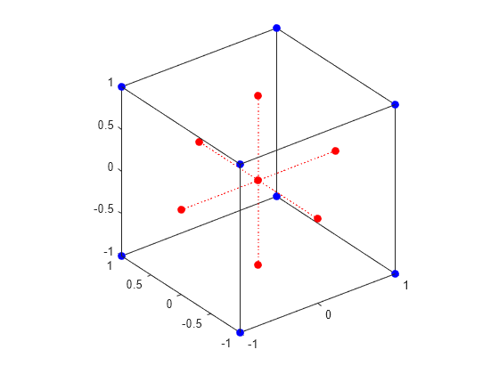
Create a three-factor central composite design with the faced type.

[dCC,blocks] = ccdesign(3,Type="faced")
dCC = 24×3

    -1    -1    -1
    -1    -1     1
    -1     1    -1
    -1     1     1
     1    -1    -1
     1    -1     1
     1     1    -1
     1     1     1
    -1     0     0
     1     0     0
      ⋮

blocks = 24×1

     1
     1
     1
     1
     1
     1
     1
     1
     2
     2
      ⋮

Visualize the design. Display the runs in the first block with blue points, and the runs in the second block with red points.

plot3(dCC(blocks == 1,1),dCC(blocks==1,2),dCC(blocks==1,3),"bo", ...
         MarkerFaceColor="b")
hold on
plot3(dCC(blocks == 2,1),dCC(blocks==2,2),dCC(blocks==2,3),"ro", ...
         MarkerFaceColor="r")
set(gca,Box="on",BoxStyle="full")
line([0 0],[0,0],[-1 1],Color="r",LineStyle=":")
line([-1 1],[0,0],[0 0],Color="r",LineStyle=":")
line([0 0],[-1,1],[0 0],Color="r",LineStyle=":")
axis square equal
hold off

Figure contains an axes object. The axes object contains 5 objects of type line. One or more of the lines displays its values using only markers

The coordinates of each point represent the factor settings of a run in the design. Because the design has the faced type, each star point is located on a face of the cube.

Input Arguments

collapse all

Number of factors in the design, specified as an integer scalar in the range [2,26].

Example: 3

Data Types: single | double

Name-Value Arguments

Specify optional pairs of arguments as Name1=Value1,...,NameN=ValueN, where Name is the argument name and Value is the corresponding value. Name-value arguments must appear after other arguments, but the order of the pairs does not matter.

Example: ccdesign(3,Center=2) creates a central composite design for three factors that contains two center points.

Number of center points in the design, specified as a nonnegative integer, "uniform", or "orthogonal". If you specify center="uniform", the function selects the number of center points needed for a design with uniform precision. If you specify center="orthogonal" (the default), the function selects the number of center points needed for an orthogonal design.

Example: Center=3

Data Types: single | double | string array

Fractional design index, specified as an integer scalar in the range [0,4]. The allowable values of fraction depend on the value of n. For example, you cannot specify a nonzero value of fraction if n ≤ 4. If fraction > 0, the software generates a design that is (0.5)^fraction of the full factorial cube. The default value of fraction depends on n.

Number of FactorsDefault Value of fractionDesign Fraction
n ≤ 4 or n > 110Entire cube
5 ≤ n ≤ 711/2 of cube
8 ≤ n ≤ 921/4 of cube
n = 1031/8 of cube
n = 1141/16 of cube

Example: Fraction=3

Data Types: single | double

Maximum number of points per block, specified as a positive integer. The default value is Inf.

Example: BlockSize=3

Data Types: single | double

Type of central composite design, specified as "circumscribed", "inscribed", or "faced". The inscribed design is the same as circumscribed, but with all factor values scaled by a factor K=(2^(n – fraction))^(–0.25). The faced design is the same as circumscribed, but with only the star factor values scaled by K. For more information about central composite design types, see Introduction to Response Surface Designs.

Example: Type="faced"

Data Types: single | double

Output Arguments

collapse all

Central composite design for n factors, returned as a numeric matrix of size m-by-n, where m is the number of runs (points) in the design. Each row of dCC contains the settings of all factors for that run. The factor values are normalized so that the cube points in the design have values between –1 and 1.

Block numbers for each run, returned as an m-by-1 numeric vector, where m is the number of runs in the design. The blocks indicate the runs to measure under similar conditions in order to minimize the effect of inter-block differences on the parameter estimates. For more information, see [2].

References

[1] Box, G. E. P., and K. B. Wilson. "On the Experimental Attainment of Optimum Conditions." Journal of the Royal Statistical Society: Series B (Methodological) 13, no. 1 (January 1951): 1–38. https://doi.org/10.1111/j.2517-6161.1951.tb00067.x.

[2] Box, G. E. P., W. G. Hunter, and J. S. Hunter. Statistics for Experimenters. Hoboken, NJ: Wiley-Interscience, 1978.

[3] Box, G. E. P., W. G. Hunter, and J. S. Hunter. "Multi-Factor Experimental Designs for Exploring Response Surfaces." Annals of Mathematical Statistics 28, no. 1 (March 1957): 195–241. https://doi.org/10.1214/aoms/1177707047.

Version History

Introduced before R2006a