Code Generation for Anomaly Detection
This example shows how to generate single-precision code that detects anomalies in data using a trained isolation forest model or one-class support vector machine (OCSVM).
The isanomaly function of isolationForest and the predict function for ClassificationSVM support code generation. These object functions require a trained model object, but the -args option of codegen (MATLAB Coder) does not accept these objects. Work around this limitation by using saveLearnerForCoder and loadLearnerForCoder as described in this example.
This flow chart shows the code generation workflow for anomaly detection.
![]()
After you train a model, save the trained model by using saveLearnerForCoder. Define an entry-point function that loads the saved model by using loadLearnerForCoder and calls the object function. Then generate code for the entry-point function by using codegen, and verify the generated code. For a more detailed code generation workflow example, see Code Generation for Prediction of Machine Learning Model at Command Line.
Load Data
Load the lidar scan data set, which contains the coordinates of objects surrounding a vehicle, stored as a collection of 3-D points.
load("lidar_subset.mat")
loc = lidar_subset;
To highlight the environment around the vehicle, set the region of interest to span 20 meters to the left and right of the vehicle, 20 meters in front and back of the vehicle, and the area above the surface of the road.
xBound = 20; % in meters
yBound = 20; % in meters
zLowerBound = 0; % in meters
Crop the data to contain only points within the specified region.
indices = loc(:,1) <= xBound & loc(:,1) >= -xBound ...
    & loc(:,2) <= yBound & loc(:,2) >= -yBound ...
    & loc(:,3) > zLowerBound;
loc = loc(indices,:);
whos loc
  Name          Size             Bytes  Class     Attributes

  loc       19070x3             228840  single
loc is a single-precision matrix containing 19,070 samples of 3-D points.
Visualize the data as a 2-D scatter plot. Annotate the plot to highlight the vehicle.
scatter(loc(:,1),loc(:,2),".");
annotation("ellipse",[0.48 0.48 .1 .1],Color="red")
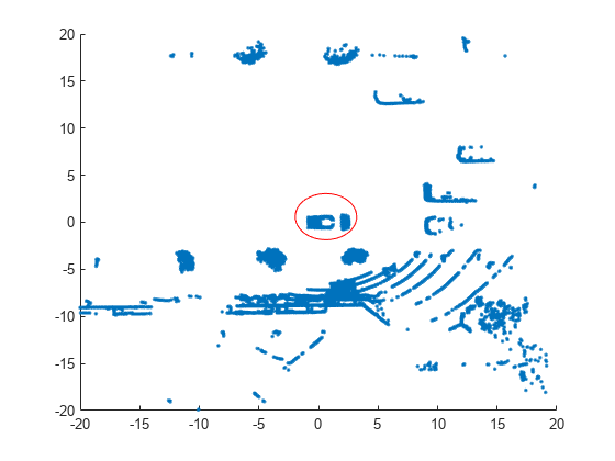
The center of the set of points (circled in red) contains the roof and hood of the vehicle. All other points are obstacles.
Assume that the fraction of outliers in the data is 0.05.
contaminationFraction = single(0.05);
Code Generation for Isolation Forest
Train Isolation Forest Model
Train an isolation forest model by using the iforest function. Specify the fraction of outliers (ContaminationFraction) as 0.05.
rng("default") % For reproducibility
[forest,tf_forest,s_forest] = iforest(loc,ContaminationFraction=contaminationFraction);
forest is an IsolationForest object. iforest also returns the anomaly indicators (tf_forest) and anomaly scores (s_forest) for the data (loc). iforest determines the score threshold value (forest.ScoreThreshold) so that the function detects the specified fraction of observations as outliers.
Save Model Using saveLearnerForCoder
Save the model object to the file IsolationForestModel.mat by using saveLearnerForCoder.
ForestMdlFileName = "IsolationForestModel";
saveLearnerForCoder(forest,ForestMdlFileName)
saveLearnerForCoder saves the object to the MATLAB® binary file IsolationForestModel.mat as a structure array in the current folder.
Define Entry-Point Function
Define an entry-point function that returns anomaly indicators and anomaly scores for the input data. Within the function, load a single-precision model by using loadLearnerForCoder, and then pass the loaded model to isanomaly.
type myIsanomaly.m % Display contents of myIsanomaly.m file
function varargout = myIsanomaly(MdlFileName,x,varargin) %#codegen
%MYISANOMALY Entry-point function for anomaly detection
% This function supports only the example Code Generation for Anomaly
% Detection and might change in a future release.
% This function detects anomalies in new observations x using the saved
% anomaly detection model in the MdlFileName file.
Mdl = loadLearnerForCoder(MdlFileName,DataType="single");
[varargout{1:nargout}] = isanomaly(Mdl,x,varargin{:});
end
Generate Code
Specify the input argument types of myIsanomaly using a 4-by-1 cell array. Assign each input argument type of the entry-point function to each cell. Specify the data type and exact input array size by using an example value that represents the set of values with a certain data type and array size.
ARGS = cell(4,1);
p = numel(forest.PredictorNames);
ARGS{1} = coder.Constant(ForestMdlFileName);
ARGS{2} = coder.typeof(single(0),[Inf,p],[1,0]);
ARGS{3} = coder.Constant("ScoreThreshold");
ARGS{4} = single(0.5);
The second input of myIsanomaly is a variable-size input. For more details on variable-size arguments, see Specify Variable-Size Arguments for Code Generation of Machine Learning Models.
Generate a MEX function from the entry-point function myIsanomaly. Specify the input argument types using the -args option and the cell array ARGS. Specify the number of output arguments in the generated entry-point function using the -nargout option.
codegen myIsanomaly -args ARGS -nargout 2
Code generation successful.
codegen generates the MEX function myIsanomaly_mex with a platform-dependent extension in the current folder.
Verify Generated Code
Detect anomalies in the training data using the generated MEX function. Compare the anomaly indicators and scores from the MEX function with those returned by iforest.
[tf_forest_MEX,s_forest_MEX] = myIsanomaly_mex(ForestMdlFileName,loc,"ScoreThreshold",single(forest.ScoreThreshold));
isequal(tf_forest,tf_forest_MEX)
ans = logical
1
max(abs(s_forest-s_forest_MEX))
ans = single
5.9605e-08
isequal returns logical 1 (true), which means all the anomaly indicators are equal. The difference in the anomaly scores is insignificant.
Code Generation for OCSVM
Train OCSVM Model
Train a support vector machine model for one-class learning by using the fitcsvm function. The function trains a model for one-class learning if the class label variable is a vector of ones. Specify the fraction of outliers (OutlierFraction) as 0.05.
MdlOCSVM = fitcsvm(loc,single(ones(size(loc,1),1)),OutlierFraction=contaminationFraction, ...
Standardize=true);MdlOCSVM is a ClassificationSVM object. Compute the outlier scores for loc by using the resubPredict function.
[~,s_OCSVM] = resubPredict(MdlOCSVM);
Negative score values indicate that the corresponding observations are outliers. Obtain the anomaly indicators.
tf_OCSVM = s_OCSVM < 0;
Save Model Using saveLearnerForCoder
Save the model object to the file SVMModel.mat by using saveLearnerForCoder.
SVMMdlFileName = "SVMModel";
saveLearnerForCoder(MdlOCSVM,SVMMdlFileName)Define Entry-Point Function
Define an entry-point function that returns anomaly indicators and anomaly scores for the input data. Within the function, load a single-precision model by using loadLearnerForCoder, and then pass the loaded model to predict to compute anomaly scores. Use the scores to find anomaly indicators.
type myIsanomalySVM.m % Display contents of myIsanomalySVM.m file
function [tf,scores] = myIsanomalySVM(MdlFileName,x,scoreThreshold) %#codegen %MYISANOMALY Entry-point function for anomaly detection % This function supports only the example Code Generation for Anomaly % Detection and might change in a future release. % This function detects anomalies in new observations x using the saved % one-class support vector machine model in the MdlFileName file. Mdl = loadLearnerForCoder(MdlFileName,DataType="single"); [~,scores] = predict(Mdl,x); tf = scores < scoreThreshold; end
Generate Code
Specify the input argument types of myIsanomalySVM using a 3-by-1 cell array.
ARGS = cell(3,1);
p = numel(MdlOCSVM.PredictorNames);
ARGS{1} = coder.Constant(SVMMdlFileName);
ARGS{2} = coder.typeof(single(0),[Inf,p],[1,0]);
ARGS{3} = single(0);Generate a MEX function from the entry-point function myIsanomalySVM.
codegen myIsanomalySVM -args ARGS -nargout 2
Code generation successful.
Verify Generated Code
Detect anomalies in the training data using the generated MEX function. Compare the anomaly indicators and scores from the MEX function with those returned by resubPredict.
[tf_OCSVM_MEX,s_OCSVM_MEX] = myIsanomalySVM_mex(SVMMdlFileName,loc,single(0));
isequal(tf_OCSVM,tf_OCSVM_MEX)
ans = logical
   1
max(abs(s_OCSVM-s_OCSVM_MEX))
ans = single

0.0130
isequal returns logical 1 (true), which means all the anomaly indicators are equal. The difference in the anomaly scores is acceptable because the average score (mean(s_OCSVM)) is around 700. You see some differences in the scores when you use the Gaussian kernel, which is the default for one-class learning.
Compare Detected Outliers
Plot the normal points and outliers detected in the isolation forest model and one-class SVM model.
tiledlayout(2,1)
nexttile
gscatter(loc(:,1),loc(:,2),tf_forest)
legend("Normal Points","Outliers")
title("Isolation Forest")
nexttile
gscatter(loc(:,1),loc(:,2),tf_OCSVM)
legend("Normal Points","Outliers")
title("One-Class SVM")
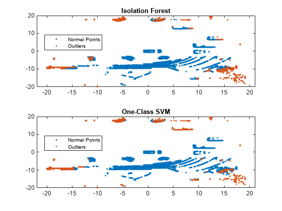
The outliers identified by the two methods are similar to each other. Compute the fraction of the same identifiers in the outputs for both methods.
mean(tf_forest == tf_OCSVM)
ans =
0.9732
See Also
codegen (MATLAB Coder) | iforest | isanomaly | fitcsvm | predict