coxphfit

Cox proportional hazards regression

Syntax

b = coxphfit(X,T)

b = coxphfit(X,T,Name,Value)

[b,logl,H,stats]
= coxphfit(___)

Description

b = coxphfit(X,T) returns a p-by-1 vector, b, of coefficient estimates for a Cox proportional hazards regression of the observed responses T on the predictors X, where T is either an n-by-1 vector or an n-by-2 matrix, and X is an n-by-p matrix.

The model does not include a constant term, and X cannot contain a column of 1s.

example

b = coxphfit(X,T,Name,Value) returns a vector of coefficient estimates, with additional options specified by one or more Name,Value pair arguments.

example

[b,logl,H,stats] = coxphfit(___) also returns the loglikelihood, logl, a structure, stats, that contains additional statistics, and a two-column matrix, H, that contains the T values in the first column and the estimated baseline cumulative hazard, in the second column. You can use any of the input arguments in the previous syntaxes.

example

Examples

collapse all

Use Cox Proportional Hazards Regression to Model Lifetime of Light Bulbs

Open Live Script

Load the sample data.

load('lightbulb.mat');

The first column of the light bulb data has the lifetime (in hours) of two different types of bulbs. The second column has the binary variable indicating whether the bulb is fluorescent or incandescent. 0 indicates that the bulb is fluorescent, and 1 indicates that it is incandescent. The third column contains the censorship information, where 0 indicates the bulb was observed until failure, and 1 indicates the bulb was censored.

Fit a Cox proportional hazards model for the lifetime of the light bulbs, also accounting for censoring. The predictor variable is the type of bulb.

b = coxphfit(lightbulb(:,2),lightbulb(:,1), ...
'Censoring',lightbulb(:,3))

b = 
4.7262

The estimate of the hazard ratio is $e^{b}$ = 112.8646. This means that the hazard for the incandescent bulbs is 112.86 times the hazard for the fluorescent bulbs.

Change Algorithm Parameters for Cox Proportional Hazards Model

Open Live Script

Load the sample data.

load('lightbulb.mat');

The first column of the data has the lifetime (in hours) of two types of bulbs. The second column has the binary variable indicating whether the bulb is fluorescent or incandescent. 1 indicates that the bulb is fluorescent and 0 indicates that it is incandescent. The third column contains the censorship information, where 0 indicates the bulb is observed until failure, and 1 indicates the item (bulb) is censored.

Fit a Cox proportional hazards model, also accounting for censoring. The predictor variable is the type of bulb.

b = coxphfit(lightbulb(:,2),lightbulb(:,1),...
'Censoring',lightbulb(:,3))

b = 
4.7262

Display the default control parameters for the algorithm coxphfit uses to estimate the coefficients.

statset('coxphfit')

ans = struct with fields:
          Display: 'off'
      MaxFunEvals: 200
          MaxIter: 100
           TolBnd: []
           TolFun: 1.0000e-08
       TolTypeFun: []
             TolX: 1.0000e-08
         TolTypeX: []
          GradObj: []
         Jacobian: []
        DerivStep: []
      FunValCheck: []
           Robust: []
     RobustWgtFun: []
           WgtFun: []
             Tune: []
      UseParallel: []
    UseSubstreams: []
          Streams: {}
        OutputFcn: []

Save the options under a different name and change how the results will be displayed and the maximum number of iterations, Display and MaxIter.

coxphopt = statset('coxphfit');
coxphopt.Display = 'final';
coxphopt.MaxIter = 50;

Run coxphfit with the new algorithm parameters.

b = coxphfit(lightbulb(:,2),lightbulb(:,1),...
'Censoring',lightbulb(:,3),'Options',coxphopt)

Successful convergence: Norm of gradient less than OPTIONS.TolFun

b = 
4.7262

coxphfit displays a report on the final iteration. Changing the maximum number of iterations did not affect the coefficient estimate.

Fit and Compare Cox and Weibull Survivor Functions

Open Live Script

Generate Weibull data depending on predictor X.

rng('default') % for reproducibility
X = 4*rand(100,1);
A = 50*exp(-0.5*X); 
B = 2;
y = wblrnd(A,B);

The response values are generated from a Weibull distribution with a scale parameter depending on the predictor variable X and a shape parameter of 2.

Fit a Cox proportional hazards model.

[b,logL,H,stats] = coxphfit(X,y);
[b logL]

ans = 1×2

    0.9409 -331.1479

The coefficient estimate is 0.9409 and the log likelihood value is –331.1479.

Request the model statistics.

stats

stats = struct with fields:
                    covb: 0.0158
                    beta: 0.9409
                      se: 0.1256
                       z: 7.4889
                       p: 6.9462e-14
                   csres: [100x1 double]
                  devres: [100x1 double]
                 martres: [100x1 double]
                  schres: [100x1 double]
                 sschres: [100x1 double]
                  scores: [100x1 double]
                 sscores: [100x1 double]
    LikelihoodRatioTestP: 6.6613e-16

The covariance matrix of the coefficient estimates, covb, contains only one value, which is equal to the variance of the coefficient estimate in this example. The coefficient estimate, beta, is the same as b and is equal to 0.9409. The standard error of the coefficient estimate, se, is 0.1256, which is the square root of the variance 0.0158. The $z$ -statistic, z, is beta/se = 0.9409/0.1256 = 7.4880. The p-value, p, indicates that the effect of X is significant.

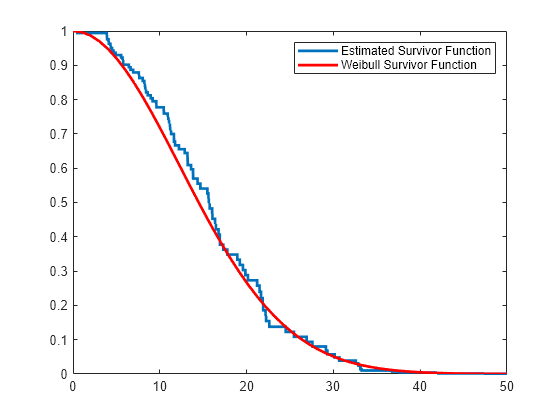
Plot the Cox estimate of the baseline survivor function together with the known Weibull function.

stairs(H(:,1),exp(-H(:,2)),'LineWidth',2)
xx = linspace(0,100);
line(xx,1-wblcdf(xx,50*exp(-0.5*mean(X)),B),'color','r','LineWidth',2)
xlim([0,50])
legend('Estimated Survivor Function','Weibull Survivor Function')

Figure contains an axes object. The axes object contains 2 objects of type stair, line. These objects represent Estimated Survivor Function, Weibull Survivor Function.

The fitted model gives a close estimate to the survivor function of the actual distribution.

Input Arguments

collapse all

`X` — Observations on predictor variables
matrix

Observations on predictor variables, specified as an n-by-p matrix of p predictors for each of n observations.

The model does not include a constant term, thus X cannot contain a column of 1s.

If X, T, or the value of 'Frequency' or 'Strata' contain NaN values, then coxphfit removes rows with NaN values from all data when fitting a Cox model.

Data Types: double

`T` — Time-to-event data
vector | two-column matrix

Time-to-event data, specified as an n-by-1 vector or a two-column matrix.

When T is an n-by-1 vector, it represents the event time of right-censored time-to-event data.
When T is an n-by-2 matrix, each row represents the risk interval (start,stop] in the counting process format for time-dependent covariates. The first column is the start time and the second column is the stop time. For an example, see Cox Proportional Hazards Model with Time-Dependent Covariates.

If X, T, or the value of 'Frequency' or 'Strata' contain NaN values, then coxphfit removes rows with NaN values from all data when fitting a Cox model.

Data Types: single | double

Name-Value Arguments

Specify optional pairs of arguments as Name1=Value1,...,NameN=ValueN, where Name is the argument name and Value is the corresponding value. Name-value arguments must appear after other arguments, but the order of the pairs does not matter.

Before R2021a, use commas to separate each name and value, and enclose Name in quotes.

Example: 'Baseline',0,'Censoring',censoreddata,'Frequency',freq specifies that coxphfit calculates the baseline hazard rate relative to 0, considering the censoring information in the vector censoreddata, and the frequency of observations on T and X given in the vector freq.

`B0` — Coefficient initial values
`0.01/std(X)` (default) | numeric vector

Coefficient initial values, specified as the comma-separated value consisting of 'B0' and a numeric vector.

Data Types: double

`Baseline` — `X` values at which to compute the baseline hazard
`mean(X)` (default) | scalar value

X values at which to compute the baseline hazard, specified as the comma-separated pair consisting of 'Baseline' and a scalar value.

The default is mean(X), so the hazard rate at X is h(t)*exp((X-mean(X))*b). Enter 0 to compute the baseline relative to 0, so the hazard rate at X is h(t)*exp(X*b). Changing the baseline does not affect the coefficient estimates, but the hazard ratio changes.

Example: 'Baseline',0

Data Types: double

`Censoring` — Indicator for censoring
array of 0s (default) | array of 0s and 1s

Indicator for censoring, specified as the comma-separated pair consisting of 'Censoring' and a Boolean array of the same size as T. Use 1 for observations that are right censored and 0 for observations that are fully observed. The default is all observations are fully observed. For an example, see Cox Proportional Hazards Model for Censored Data.

Example: 'Censoring',cens

Data Types: logical

`Frequency` — Frequency or weights of observations
array of 1s (default) | vector of nonnegative scalar values

Frequency or weights of observations, specified as the comma-separated pair consisting of 'Frequency' and an array that is the same size as T containing nonnegative scalar values. The array can contain integer values corresponding to frequencies of observations or nonnegative values corresponding to observation weights.

If X, T, or the value of 'Frequency' or 'Strata' contain NaN values, then coxphfit removes rows with NaN values from all data when fitting a Cox model.

The default is 1 per row of X and T.

Example: 'Frequency',w

Data Types: double

`Strata` — Stratification variables
`[]` (default) | matrix of real values

Stratification variables, specified as the comma-separated pair consisting of a matrix of real values. The matrix must have the same number of rows as T, with each row corresponding to an observation.

If X, T, or the value of 'Frequency' or 'Strata' contain NaN values, then coxphfit removes rows with NaN values from all data when fitting a Cox model.

The default, [], is no stratification variable.

Example: 'Strata',Gender

Data Types: single | double

`Ties` — Method to handle tied failure times
`'breslow'` (default) | `'efron'`

Method to handle tied failure times, specified as the comma-separated pair consisting of 'Ties' and either 'breslow' (Breslow's method) or 'efron' (Efron's method).

Example: 'Ties','efron'

`Options` — Algorithm control parameters
structure

Algorithm control parameters for the iterative algorithm used to estimate b, specified as the comma-separated pair consisting of 'Options' and a structure. A call to statset creates this argument. For parameter names and default values, type statset('coxphfit'). You can set the options under a new name and use that in the name-value pair argument.

Example: 'Options',statset('coxphfit')

Output Arguments

collapse all

`b` — Coefficient estimates
vector

Coefficient estimates for a Cox proportional hazards regression, returned as a p-by-1 vector.

`logl` — Loglikelihood
scalar

Loglikelihood of the fitted model, returned as a scalar.

You can use log likelihood values to compare different models and assess the significance of effects of terms in the model.

`H` — Estimated baseline cumulative hazard
two-column matrix | (2+k) column matrix

Estimated baseline cumulative hazard rate evaluated at T values, returned as one of the following.

If the model is unstratified, then H is a two-column matrix. The first column of the matrix contains T values, and the second column contains cumulative hazard rate estimates.
If the model is stratified, then H is a (2+k) column matrix, where the last k columns correspond to the stratification variables using the Strata name-value pair argument.

`stats` — Coefficient statistics
structure

Coefficient statistics, returned as a structure that contains the following fields.

`beta`	Coefficient estimates (same as `b`)
`se`	Standard errors of coefficient estimates, `b`
`z`	z-statistics for `b` (that is, `b` divided by standard error)
`p`	p-values for `b`
`covb`	Estimated covariance matrix for `b`
`csres`	Cox-Snell residuals
`devres`	Deviance residuals
`martres`	Martingale residuals
`schres`	Schoenfeld residuals
`sschres`	Scaled Schoenfeld residuals
`scores`	Score residuals
`sscores`	Scaled score residuals

coxphfit returns the Cox-Snell, martingale, and deviance residuals as a column vector with one row per observation. It returns the Schoenfeld, scaled Schoenfeld, score, and scaled score residuals as matrices of the same size as X. Schoenfeld and scaled Schoenfeld residuals of censored data are NaNs.

More About

collapse all

Cox Proportional Hazards Regression

Cox proportional hazards regression is a semiparametric method for adjusting survival rate estimates to remove the effect of confounding variables and to quantify the effect of predictor variables. The method represents the effects of explanatory and confounding variables as a multiplier of a common baseline hazard function, h₀(t).

For a baseline relative to 0, this model corresponds to

$h (X_{i}, t) = h_{0} (t) \exp [\sum_{j = 1}^{p} x_{i j} b_{j}],$

where $X_{i} = (x_{i 1}, x_{i 2}, \dots, x_{i p})$ is the predictor variable for the ith subject, h(X_i,t) is the hazard rate at time t for X_i, and h₀(t) is the baseline hazard rate function. The baseline hazard function is the nonparametric part of the Cox proportional hazards regression function, whereas the impact of the predictor variables is a loglinear regression. The assumption is that the baseline hazard function depends on time, t, but the predictor variables do not depend on time. See Cox Proportional Hazards Model for details, including the extensions for stratification and time-dependent variables, tied events, and observation weights.

Algorithms

If you want to compute the baseline cumulative hazard rate (H) for a stratum, the input data for the stratum must contain at least one fully observed observation. If a stratum has only censored observations, the output H includes a row with NaNs in the first two columns and the stratum information in the remaining columns.
Before R2022a: If a stratum has only censored observations, H includes a row of zeros and no stratum information.

References

[1] Cox, D.R., and D. Oakes. Analysis of Survival Data. London: Chapman & Hall, 1984.

[2] Lawless, J. F. Statistical Models and Methods for Lifetime Data. Hoboken, NJ: Wiley-Interscience, 2002.

[3] Kleinbaum, D. G., and M. Klein. Survival Analysis. Statistics for Biology and Health. 2nd edition. Springer, 2005.

Extended Capabilities

C/C++ Code Generation
Generate C and C++ code using MATLAB® Coder™.

Usage notes and limitations:

X can be a single- or double-precision matrix and can be variable-size.
The value of the 'Ties' name-value pair argument must be a compile-time constant. For example, to use Efron's method to handle tied failure times, include {coder.Constant('Ties'),coder.Constant('efron')} in the -args value of codegen (MATLAB Coder).
Names in name-value arguments must be compile-time constants.

For more information on code generation, see Introduction to Code Generation and General Code Generation Workflow.

Version History

Introduced before R2006a

expand all

R2022a: Return stratum information for a stratum that has only censored observations

If a stratum has only censored observations, the output H includes a row with NaNs in the first two columns and the stratum information in the remaining columns. In previous releases, H included a row of zeros and no stratum information.

coxphfit

Syntax

Description

Examples

Use Cox Proportional Hazards Regression to Model Lifetime of Light Bulbs

Change Algorithm Parameters for Cox Proportional Hazards Model

Fit and Compare Cox and Weibull Survivor Functions

Input Arguments

`X` — Observations on predictor variables
matrix

`T` — Time-to-event data
vector | two-column matrix

Name-Value Arguments

`B0` — Coefficient initial values
`0.01/std(X)` (default) | numeric vector

`Baseline` — `X` values at which to compute the baseline hazard
`mean(X)` (default) | scalar value

`Censoring` — Indicator for censoring
array of 0s (default) | array of 0s and 1s

`Frequency` — Frequency or weights of observations
array of 1s (default) | vector of nonnegative scalar values

`Strata` — Stratification variables
`[]` (default) | matrix of real values

`Ties` — Method to handle tied failure times
`'breslow'` (default) | `'efron'`

`Options` — Algorithm control parameters
structure

Output Arguments

`b` — Coefficient estimates
vector

`logl` — Loglikelihood
scalar

`H` — Estimated baseline cumulative hazard
two-column matrix | (2+k) column matrix

`stats` — Coefficient statistics
structure

More About

Cox Proportional Hazards Regression

Algorithms

References

Extended Capabilities

C/C++ Code Generation
Generate C and C++ code using MATLAB® Coder™.

Version History

R2022a: Return stratum information for a stratum that has only censored observations

See Also

Topics

coxphfit

Syntax

Description

Examples

Use Cox Proportional Hazards Regression to Model Lifetime of Light Bulbs

Change Algorithm Parameters for Cox Proportional Hazards Model

Fit and Compare Cox and Weibull Survivor Functions

Input Arguments

X — Observations on predictor variables matrix

T — Time-to-event data vector | two-column matrix

Name-Value Arguments

B0 — Coefficient initial values 0.01/std(X) (default) | numeric vector

Baseline — X values at which to compute the baseline hazard mean(X) (default) | scalar value

Censoring — Indicator for censoring array of 0s (default) | array of 0s and 1s

Frequency — Frequency or weights of observations array of 1s (default) | vector of nonnegative scalar values

Strata — Stratification variables [] (default) | matrix of real values

Ties — Method to handle tied failure times 'breslow' (default) | 'efron'

Options — Algorithm control parameters structure

Output Arguments

b — Coefficient estimates vector

logl — Loglikelihood scalar

H — Estimated baseline cumulative hazard two-column matrix | (2+k) column matrix

stats — Coefficient statistics structure

More About

Cox Proportional Hazards Regression

Algorithms

References

Extended Capabilities

C/C++ Code Generation Generate C and C++ code using MATLAB® Coder™.

Version History

R2022a: Return stratum information for a stratum that has only censored observations

See Also

Topics

`X` — Observations on predictor variables
matrix

`T` — Time-to-event data
vector | two-column matrix

`B0` — Coefficient initial values
`0.01/std(X)` (default) | numeric vector

`Baseline` — `X` values at which to compute the baseline hazard
`mean(X)` (default) | scalar value

`Censoring` — Indicator for censoring
array of 0s (default) | array of 0s and 1s

`Frequency` — Frequency or weights of observations
array of 1s (default) | vector of nonnegative scalar values

`Strata` — Stratification variables
`[]` (default) | matrix of real values

`Ties` — Method to handle tied failure times
`'breslow'` (default) | `'efron'`

`Options` — Algorithm control parameters
structure

`b` — Coefficient estimates
vector

`logl` — Loglikelihood
scalar

`H` — Estimated baseline cumulative hazard
two-column matrix | (2+k) column matrix

`stats` — Coefficient statistics
structure

C/C++ Code Generation
Generate C and C++ code using MATLAB® Coder™.