Kaplan-Meier Method
The Statistics and Machine Learning Toolbox™ function ecdf produces
the empirical cumulative hazard, survivor, and cumulative distribution
functions by using the Kaplan-Meier nonparametric method. The Kaplan-Meier
estimator for the survivor function is also called the product-limit
estimator.
The Kaplan-Meier method uses survival data summarized in life
tables. Life tables order data according to ascending failure times,
but you don’t have to enter the failure/survival times in an
ordered manner to use ecdf.
A life table usually consists of:
Failure times
Number of items failed at a time/time period
Number of items censored at a time/time period
Number of items at risk at the beginning of a time/time period
The number at risk is the total number of survivors at the beginning of each period. The number at risk at the beginning of the first period is all individuals in the lifetime study. At the beginning of each remaining period, the number at risk is reduced by the number of failures plus individuals censored at the end of the previous period.
This life table shows fictitious survival data. At the beginning of the first failure time, there are seven items at risk. At time 4, three fail. So at the beginning of time 7, there are four items at risk. Only one fails at time 7, so the number at risk at the beginning of time 11 is three. Two fail at time 11, so at the beginning of time 12, the number at risk is one. The remaining item fails at time 12.
| Failure Time (t) | Number Failed | Number at Risk |
|---|---|---|
| 4 | 3 | 7 |
| 7 | 1 | 4 |
| 11 | 2 | 3 |
| 12 | 1 | 1 |
You can estimate the hazard, cumulative hazard, survival, and cumulative distribution functions using the life tables as described next.
Cumulative Hazard Rate (Failure Rate)
The hazard rate at each period is the number of failures in the given period divided by the number of surviving individuals at the beginning of the period (number at risk).
| Failure Time (t) | Hazard Rate (h(t)) | Cumulative Hazard Rate |
|---|---|---|
| 0 | 0 | 0 |
| t1 | d1/r1 | d1/r1 |
| t2 | d2/r2 | h(t1) + d2/r2 |
| ... | ... | ... |
| tn | dn/rn | h(tn – 1) + dn/rn |
Survival Probability
For each period, the survival probability is the product of the complement of hazard rates. The initial survival probability at the beginning of the first time period is 1. If the hazard rate for the each period is h(ti), then the survivor probability is as shown.
| Time (t) | Survival Probability (S(t)) |
|---|---|
| 0 | 1 |
| t1 | 1*(1 – h(t1)) |
| t2 | S(t1)*(1 – h(t2)) |
| ... | ... |
| tn | S(tn – 1)*(1 – h(tn)) |
Cumulative Distribution Function
Because the cumulative distribution function (cdf) and the survivor function are complements of each other, you can find the cdf from the life tables using F(t) = 1 – S(t).
You can compute the cumulative hazard rate, survival rate, and cumulative distribution function for the simulated data in the first table on this page as follows.
| t | Number Failed (d) | Number at Risk (r) | Hazard Rate | Survival Probability | Cumulative Distribution Function |
|---|---|---|---|---|---|
| 4 | 3 | 7 | 3/7 | 1 – 3/7 = 4/7 = 0.5714 | 0.4286 |
| 7 | 1 | 4 | 1/4 | 4/7*(1 – 1/4) = 3/7 = .4286 | 0.5714 |
| 11 | 2 | 3 | 2/3 | 3/7*(1 – 2/3) = 1/7 = 0.1429 | 0.8571 |
| 12 | 1 | 1 | 1/1 | 1/7*(1 – 1) = 0 | 1 |
This rates in this example are based on the discrete failure times, and hence the calculations do not necessarily follow the derivative-based definition in What Is Survival Analysis?
Here is how you can enter the data and calculate these measures
using ecdf. The data does not necessarily have
to be in ascending order. Suppose the failure times are stored in
an array y.
y = [4 7 11 12];
freq = [3 1 2 1];
[f,x] = ecdf(y,'frequency',freq)
f =
0
0.4286
0.5714
0.8571
1.0000
x =
4
4
7
11
12When you have censored data, the life table might look like the following:
| Time (t) | Number failed (d) | Censoring | Number at Risk (r) | Hazard Rate | Survival Probability | Cumulative Distribution Function |
|---|---|---|---|---|---|---|
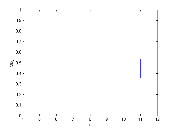
| 4 | 2 | 1 | 7 | 2/7 | 1 – 2/7 = 0.7143 | 0.2857 |
| 7 | 1 | 0 | 4 | 1/4 | 0.7143*(1 – 1/4) = 0.5357 | 0.4643 |
| 11 | 1 | 1 | 3 | 1/3 | 0.5357*(1 – 1/3) = 0.3571 | 0.6429 |
| 12 | 1 | 0 | 1 | 1/1 | 0.3571*(1 – 1) = 0 | 1.0000 |
At any given time, the censored items are also considered in the total of number at risk, and the hazard rate formula is based on the number failed and the total number at risk. While updating the number at risk at the beginning of each period, the total number failed and censored in the previous period is reduced from the number at risk at the beginning of that period.
While using ecdf, you must also enter the
censoring information using an array of binary variables. Enter 1
for censored data, and enter 0 for exact failure time.
y = [4 4 4 7 11 11 12];
cens = [0 1 0 0 1 0 0];
[f,x] = ecdf(y,'censoring',cens)
f =
0
0.2857
0.4643
0.6429
1.0000
x =
4
4
7
11
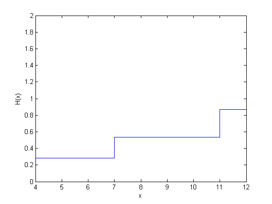
12ecdf, by default, produces the cumulative
distribution function values. You have to specify the survivor function
or the hazard function using optional name-value pair arguments. You
can also plot the results as follows.
figure()
ecdf(y,'censoring',cens,'function','survivor');

figure()
ecdf(y,'censoring',cens,'function','cumulative hazard');

References
[1] Cox, D. R., and D. Oakes. Analysis of Survival Data. London: Chapman & Hall, 1984.
[2] Lawless, J. F. Statistical Models and Methods for Lifetime Data. Hoboken, NJ: Wiley-Interscience, 2002.
[3] Kleinbaum, D. G., and M. Klein. Survival Analysis. Statistics for Biology and Health. 2nd edition. Springer, 2005.