Main Content

report

Generate fairness metrics report

Since R2022b

    Description

    example

    metricsTbl = report(evaluator) generates a table metricsTbl that contains the bias metrics stored in the BiasMetrics property of the fairnessMetrics object evaluator.

    example

    metricsTbl = report(evaluator,Name=Value) specifies additional options using one or more name-value arguments. You can specify bias metrics and group metrics to include in metricsTbl by using the BiasMetrics and GroupMetrics name-value arguments, respectively.

    Examples

    collapse all

    Compute fairness metrics for predicted labels with respect to sensitive attributes by creating a fairnessMetrics object. Then, create a metrics table for specified fairness metrics by using the BiasMetrics and GroupMetrics name-value arguments of the report function.

    Load the sample data census1994, which contains the training data adultdata and the test data adulttest. The data sets consist of demographic information from the US Census Bureau that can be used to predict whether an individual makes over $50,000 per year. Preview the first few rows of the training data set.

    load census1994
    head(adultdata)
        age       workClass          fnlwgt      education    education_num       marital_status           occupation        relationship     race      sex      capital_gain    capital_loss    hours_per_week    native_country    salary
        ___    ________________    __________    _________    _____________    _____________________    _________________    _____________    _____    ______    ____________    ____________    ______________    ______________    ______
    
        39     State-gov                77516    Bachelors         13          Never-married            Adm-clerical         Not-in-family    White    Male          2174             0                40          United-States     <=50K 
        50     Self-emp-not-inc         83311    Bachelors         13          Married-civ-spouse       Exec-managerial      Husband          White    Male             0             0                13          United-States     <=50K 
        38     Private             2.1565e+05    HS-grad            9          Divorced                 Handlers-cleaners    Not-in-family    White    Male             0             0                40          United-States     <=50K 
        53     Private             2.3472e+05    11th               7          Married-civ-spouse       Handlers-cleaners    Husband          Black    Male             0             0                40          United-States     <=50K 
        28     Private             3.3841e+05    Bachelors         13          Married-civ-spouse       Prof-specialty       Wife             Black    Female           0             0                40          Cuba              <=50K 
        37     Private             2.8458e+05    Masters           14          Married-civ-spouse       Exec-managerial      Wife             White    Female           0             0                40          United-States     <=50K 
        49     Private             1.6019e+05    9th                5          Married-spouse-absent    Other-service        Not-in-family    Black    Female           0             0                16          Jamaica           <=50K 
        52     Self-emp-not-inc    2.0964e+05    HS-grad            9          Married-civ-spouse       Exec-managerial      Husband          White    Male             0             0                45          United-States     >50K  
    

    Each row contains the demographic information for one adult. The information includes sensitive attributes, such as age, marital_status, relationship, race, and sex. The third column flnwgt contains observation weights, and the last column salary shows whether a person has a salary less than or equal to $50,000 per year (<=50K) or greater than $50,000 per year (>50K).

    Train a classification tree using the training data set adultdata. Specify the response variable, predictor variables, and observation weights by using the variable names in the adultdata table.

    predictorNames = ["capital_gain","capital_loss","education", ...
        "education_num","hours_per_week","occupation","workClass"];
    Mdl = fitctree(adultdata,"salary", ...
        PredictorNames=predictorNames,Weights="fnlwgt");

    Predict the test sample labels by using the trained tree Mdl.

    adulttest.predictions = predict(Mdl,adulttest);

    This example evaluates the fairness of the predicted labels with respect to age and marital status. Group the age variable into four bins.

    ageGroups = ["Age<30","30<=Age<45","45<=Age<60","Age>=60"];
    adulttest.age_group = discretize(adulttest.age, ...
        [min(adulttest.age) 30 45 60 max(adulttest.age)], ...
        categorical=ageGroups);

    Compute fairness metrics for the predictions with respect to the age_group and marital_status variables by using fairnessMetrics.

    MdlEvaluator = fairnessMetrics(adulttest,"salary", ...
        SensitiveAttributeNames=["age_group","marital_status"], ...
        Predictions="predictions",ModelNames="Tree",Weights="fnlwgt");

    fairnessMetrics computes metrics for all supported bias and group metrics. Display the names of the metrics stored in the BiasMetrics and GroupMetrics properties.

    MdlEvaluator.BiasMetrics.Properties.VariableNames(4:end)'
    ans = 4x1 cell
        {'StatisticalParityDifference'  }
        {'DisparateImpact'              }
        {'EqualOpportunityDifference'   }
        {'AverageAbsoluteOddsDifference'}
    
    
    MdlEvaluator.GroupMetrics.Properties.VariableNames(4:end)'
    ans = 17x1 cell
        {'GroupCount'               }
        {'GroupSizeRatio'           }
        {'TruePositives'            }
        {'TrueNegatives'            }
        {'FalsePositives'           }
        {'FalseNegatives'           }
        {'TruePositiveRate'         }
        {'TrueNegativeRate'         }
        {'FalsePositiveRate'        }
        {'FalseNegativeRate'        }
        {'FalseDiscoveryRate'       }
        {'FalseOmissionRate'        }
        {'PositivePredictiveValue'  }
        {'NegativePredictiveValue'  }
        {'RateOfPositivePredictions'}
        {'RateOfNegativePredictions'}
        {'Accuracy'                 }


    Create a table containing fairness metrics by using the report function. Specify BiasMetrics as ["eod","aaod"] to include the equal opportunity difference (EOD) and average absolute odds difference (AAOD) metrics in the report table. fairnessMetrics computes the two metrics by using the true positive rates (TPR) and false positive rates (FPR). Specify GroupMetrics as ["tpr","fpr"] to include TPR and FPR values in the table.

    metricsTbl = report(MdlEvaluator, ...
        BiasMetrics=["eod","aaod"],GroupMetrics=["tpr","fpr"]);

    Display the fairness metrics for the sensitive attribute age_group only.

    metricsTbl(metricsTbl.SensitiveAttributeNames=="age_group",3:end)
    ans=4×5 table
          Groups      EqualOpportunityDifference    AverageAbsoluteOddsDifference    TruePositiveRate    FalsePositiveRate
        __________    __________________________    _____________________________    ________________    _________________
    
        Age<30                -0.041586                        0.044576                  0.41333             0.041053     
        30<=Age<45                    0                               0                  0.45491             0.088618     
        45<=Age<60             0.061227                        0.031446                  0.51614             0.086954     
        Age>=60                0.001949                       0.0099106                  0.45686             0.070746     


    Compute fairness metrics for true labels with respect to sensitive attributes by creating a fairnessMetrics object. Then, create a table with all supported fairness metrics by using the report function.

    Read the sample file CreditRating_Historical.dat into a table. The predictor data consists of financial ratios and industry sector information for a list of corporate customers. The response variable consists of credit ratings assigned by a rating agency.

    creditrating = readtable("CreditRating_Historical.dat");

    Because each value in the ID variable is a unique customer ID—that is, length(unique(creditrating.ID)) is equal to the number of observations in creditrating—the ID variable is a poor predictor. Remove the ID variable from the table, and convert the Industry variable to a categorical variable.

    creditrating.ID = [];
    creditrating.Industry = categorical(creditrating.Industry);

    In the Rating response variable, combine the AAA, AA, A, and BBB ratings into a category of "good" ratings, and the BB, B, and CCC ratings into a category of "poor" ratings.

    Rating = categorical(creditrating.Rating);
    Rating = mergecats(Rating,["AAA","AA","A","BBB"],"good");
    Rating = mergecats(Rating,["BB","B","CCC"],"poor");
    creditrating.Rating = Rating;

    Compute fairness metrics with respect to the sensitive attribute Industry for the labels in the Rating variable.

    evaluator = fairnessMetrics(creditrating,"Rating", ...
        SensitiveAttributeNames="Industry");

    Display the bias metrics by using the report function. By default, the report function creates a table with all bias metrics.

    report(evaluator)
    ans=12×4 table
        SensitiveAttributeNames    Groups    StatisticalParityDifference    DisparateImpact
        _______________________    ______    ___________________________    _______________
    
               Industry              1                 0.077242                  1.2632    
               Industry              2                 0.078577                  1.2678    
               Industry              3                        0                       1    
               Industry              4                 0.088718                  1.3023    
               Industry              5                 0.055526                  1.1892    
               Industry              6                -0.015004                 0.94887    
               Industry              7                 0.014489                  1.0494    
               Industry              8                 0.063476                  1.2163    
               Industry              9                  0.13948                  1.4753    
               Industry              10                 0.13865                  1.4725    
               Industry              11                0.009886                  1.0337    
               Industry              12                0.029338                     1.1    


    Create a table with all supported bias and group metrics. Specify GroupMetrics as "all" to include all group metrics.

    report(evaluator,GroupMetrics="all")
    ans=12×6 table
        SensitiveAttributeNames    Groups    StatisticalParityDifference    DisparateImpact    GroupCount    GroupSizeRatio
        _______________________    ______    ___________________________    _______________    __________    ______________
    
               Industry              1                 0.077242                  1.2632           348           0.088505   
               Industry              2                 0.078577                  1.2678           336           0.085453   
               Industry              3                        0                       1           351           0.089268   
               Industry              4                 0.088718                  1.3023           314           0.079858   
               Industry              5                 0.055526                  1.1892           341           0.086724   
               Industry              6                -0.015004                 0.94887           334           0.084944   
               Industry              7                 0.014489                  1.0494           315           0.080112   
               Industry              8                 0.063476                  1.2163           325           0.082655   
               Industry              9                  0.13948                  1.4753           328           0.083418   
               Industry              10                 0.13865                  1.4725           324           0.082401   
               Industry              11                0.009886                  1.0337           300           0.076297   
               Industry              12                0.029338                     1.1           316           0.080366   


    Train two classification models, and compare the model predictions by using fairness metrics.

    Read the sample file CreditRating_Historical.dat into a table. The predictor data consists of financial ratios and industry sector information for a list of corporate customers. The response variable consists of credit ratings assigned by a rating agency.

    creditrating = readtable("CreditRating_Historical.dat");

    Because each value in the ID variable is a unique customer ID—that is, length(unique(creditrating.ID)) is equal to the number of observations in creditrating—the ID variable is a poor predictor. Remove the ID variable from the table, and convert the Industry variable to a categorical variable.

    creditrating.ID = [];
    creditrating.Industry = categorical(creditrating.Industry);

    In the Rating response variable, combine the AAA, AA, A, and BBB ratings into a category of "good" ratings, and the BB, B, and CCC ratings into a category of "poor" ratings.

    Rating = categorical(creditrating.Rating);
    Rating = mergecats(Rating,["AAA","AA","A","BBB"],"good");
    Rating = mergecats(Rating,["BB","B","CCC"],"poor");
    creditrating.Rating = Rating;

    Train a support vector machine (SVM) model on the creditrating data. For better results, standardize the predictors before fitting the model. Use the trained model to predict labels and compute the misclassification rate for the training data set.

    predictorNames = ["WC_TA","RE_TA","EBIT_TA","MVE_BVTD","S_TA"];
    SVMMdl = fitcsvm(creditrating,"Rating", ...
        PredictorNames=predictorNames,Standardize=true);
    SVMPredictions = resubPredict(SVMMdl);
    resubLoss(SVMMdl)
    ans = 0.0872
    

    Train a generalized additive model (GAM).

    GAMMdl = fitcgam(creditrating,"Rating", ...
        PredictorNames=predictorNames);
    GAMPredictions = resubPredict(GAMMdl);
    resubLoss(GAMMdl)
    ans = 0.0542
    

    GAMMdl achieves better accuracy on the training data set.

    Compute fairness metrics with respect to the sensitive attribute Industry by using the model predictions for both models.

    predictions = [SVMPredictions,GAMPredictions];
    evaluator = fairnessMetrics(creditrating,"Rating", ...
        SensitiveAttributeNames="Industry",Predictions=predictions, ...
        ModelNames=["SVM","GAM"]);

    Display the bias metrics by using the report function.

    report(evaluator)
    ans=48×5 table
                  Metrics              SensitiveAttributeNames    Groups       SVM          GAM    
        ___________________________    _______________________    ______    _________    __________
    
        StatisticalParityDifference           Industry              1       -0.028441     0.0058208
        StatisticalParityDifference           Industry              2        -0.04014     0.0063339
        StatisticalParityDifference           Industry              3               0             0
        StatisticalParityDifference           Industry              4        -0.04905    -0.0043007
        StatisticalParityDifference           Industry              5       -0.015615     0.0041607
        StatisticalParityDifference           Industry              6        -0.03818     -0.024515
        StatisticalParityDifference           Industry              7        -0.01514      0.007326
        StatisticalParityDifference           Industry              8       0.0078632      0.036581
        StatisticalParityDifference           Industry              9       -0.013863      0.042266
        StatisticalParityDifference           Industry              10      0.0090218      0.050095
        StatisticalParityDifference           Industry              11      -0.004188      0.001453
        StatisticalParityDifference           Industry              12      -0.041572     -0.028589
        DisparateImpact                       Industry              1         0.92261         1.017
        DisparateImpact                       Industry              2         0.89078        1.0185
        DisparateImpact                       Industry              3               1             1
        DisparateImpact                       Industry              4         0.86654       0.98742
          ⋮


    Among the bias metrics, compare the equal opportunity difference (EOD) values. Create a bar graph of the EOD values by using the plot function.

    b = plot(evaluator,"eod");
    b(1).FaceAlpha = 0.2;
    b(2).FaceAlpha = 0.2;
    legend(Location="southwest")

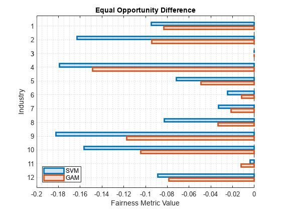
    To better understand the distributions of EOD values, plot the values using box plots.

    boxchart(evaluator.BiasMetrics.EqualOpportunityDifference, ...
        GroupByColor=evaluator.BiasMetrics.ModelNames)
    ax = gca;
    ax.XTick = [];
    ylabel("Equal Opportunity Difference")
    legend

    The EOD values for GAM are closer to 0 compared to the values for SVM.

    Input Arguments

    collapse all

    Fairness evaluator, specified as a fairnessMetrics object.

    Name-Value Arguments

    Specify optional pairs of arguments as Name1=Value1,...,NameN=ValueN, where Name is the argument name and Value is the corresponding value. Name-value arguments must appear after other arguments, but the order of the pairs does not matter.

    Example: BiasMetrics="",GroupMetrics="all" specifies to display all group metrics.

    List of bias metrics, specified as "all", [], a character vector or string scalar of a metric name, or a string array or cell array of character vectors containing more than one metric name.

    • "all" (default) — The output table metricsTbl returned by the report function includes all bias metrics in the BiasMetrics property of evaluator.

    • []metricsTbl does not include any bias metrics.

    • One or more bias metric names in the BiasMetrics property — The BiasMetrics property in evaluator and the output table metricsTbl use full names for the table variable names. However, you can use the full names or short names, as given in the following table, to specify the BiasMetrics name-value argument.

    Metric NameDescriptionEvaluation Type
    "StatisticalParityDifference" or "spd"Statistical parity difference (SPD)Data-level or model-level evaluation
    "DisparateImpact" or "di"Disparate impact (DI)Data-level or model-level evaluation
    "EqualOpportunityDifference" or "eod"Equal opportunity difference (EOD)Model-level evaluation
    "AverageAbsoluteOddsDifference" or "aaod"Average absolute odds difference (AAOD)Model-level evaluation

    The supported bias metrics depend on whether you specify predicted labels by using the Predictions argument when you create a fairnessMetrics object.

    • Data-level evaluation — If you specify true labels and do not specify predicted labels, the BiasMetrics property contains only StatisticalParityDifference and DisparateImpact.

    • Model-level evaluation — If you specify both true labels and predicted labels, the BiasMetrics property contains all metrics listed in the table.

    For definitions of the bias metrics, see Bias Metrics.

    Example: BiasMetrics=["spd","eod"]

    Data Types: char | string | cell

    Since R2023a

    Flag to display metrics in rows, specified as true or false. A true value indicates that each row of metricsTbl contains values for one fairness metric only.

    • When you perform data-level evaluation or model-level evaluation for one model, the default DisplayMetricsInRows value is false.

    • When you perform model-level evaluation for two or more models, the default DisplayMetricsInRows value is true.

    Example: DisplayMetricsInRows=false

    Data Types: logical

    List of group metrics, specified as [], "all", a character vector or string scalar of a metric name, or a string array or cell array of character vectors containing more than one metric name.

    • [] (default) — The output table metricsTbl returned by the report function does not include any group metrics.

    • "all"metricsTbl includes all group metrics in the GroupMetrics property of evaluator.

    • One or more group metric names in the GroupMetrics property — The GroupMetrics property in evaluator and the output table metricsTbl use full names for the table variable names. However, you can use the full names or short names, as given in the following table, to specify the GroupMetrics name-value argument.

    Metric NameDescriptionEvaluation Type
    "GroupCount"Group count, or number of samples in the groupData-level or model-level evaluation
    "GroupSizeRatio"Group count divided by the total number of samplesData-level or model-level evaluation
    "TruePositives" or "tp"Number of true positives (TP)Model-level evaluation
    "TrueNegatives" or "tn"Number of true negatives (TN)Model-level evaluation
    "FalsePositives" or "fp"Number of false positives (FP)Model-level evaluation
    "FalseNegatives" or "fn"Number of false negatives (FN)Model-level evaluation
    "TruePositiveRate" or "tpr"True positive rate (TPR), also known as recall or sensitivity, TP/(TP+FN)Model-level evaluation
    "TrueNegativeRate", "tnr", or "spec"True negative rate (TNR), or specificity, TN/(TN+FP)Model-level evaluation
    "FalsePositiveRate" or "fpr"False positive rate (FPR), also known as fallout or 1-specificity, FP/(TN+FP)Model-level evaluation
    "FalseNegativeRate", "fnr", or "miss"False negative rate (FNR), or miss rate, FN/(TP+FN)Model-level evaluation
    "FalseDiscoveryRate" or "fdr"False discovery rate (FDR), FP/(TP+FP)Model-level evaluation
    "FalseOmissionRate" or "for"False omission rate (FOR), FN/(TN+FN)Model-level evaluation
    "PositivePredictiveValue", "ppv", or "prec"Positive predictive value (PPV), or precision, TP/(TP+FP)Model-level evaluation
    "NegativePredictiveValue" or "npv"Negative predictive value (NPV), TN/(TN+FN)Model-level evaluation
    "RateOfPositivePredictions" or "rpp"Rate of positive predictions (RPP), (TP+FP)/(TP+FN+FP+TN)Model-level evaluation
    "RateOfNegativePredictions" or "rnp"Rate of negative predictions (RNP), (TN+FN)/(TP+FN+FP+TN)Model-level evaluation
    "Accuracy" or "accu"Accuracy, (TP+TN)/(TP+FN+FP+TN)Model-level evaluation

    The supported group metrics depend on whether you specify predicted labels by using the Predictions argument when you create a fairnessMetrics object.

    • Data-level evaluation — If you specify true labels and do not specify predicted labels, the GroupMetrics property contains only GroupCount and GroupSizeRatio.

    • Model-level evaluation — If you specify both true labels and predicted labels, the GroupMetrics property contains all metrics listed in the table.

    Example: GroupMetrics="all"

    Data Types: char | string | cell

    Since R2023a

    Names of the models to include in the report metricsTbl, specified as "all", a character vector, a string array, or a cell array of character vectors. The ModelNames value must contain names in the ModelNames property of evaluator. Using the "all" value is equivalent to specifying evaluator.ModelNames.

    Example: ModelNames="Tree"

    Example: ModelNames=["SVM","Ensemble"]

    Data Types: char | string | cell

    Output Arguments

    collapse all

    Fairness metrics, returned as a table. The format of the table depends on the type of evaluation and the DisplayMetricsInRows value.

    Evaluation TypeDisplayMetricsInRows ValuemetricsTbl Format
    Data-level evaluationfalse
    • Each row of the table contains values for one sensitive attribute group.

    • The table columns are (in order): SensitiveAttributeNames, Groups, and one column for each metric specified by the BiasMetrics and GroupMetrics name-value arguments.

    Data-level evaluationtrue
    • Each row of the table contains values for one sensitive attribute group and one fairness metric.

    • The table columns are (in order): Metrics, SensitiveAttributeNames, Groups, and Data.

    Model-level evaluationfalse
    • Each row of the table contains values for one sensitive attribute group and one model.

    • The table columns are (in order): ModelNames, SensitiveAttributeNames, Groups, and one column for each metric specified by the BiasMetrics and GroupMetrics name-value arguments.

    Model-level evaluationtrue
    • Each row of the table contains values for one sensitive attribute group and one fairness metric.

    • The table columns are (in order): Metrics, SensitiveAttributeNames, Groups, and one column for each model specified by the ModelNames name-value argument.

    More About

    collapse all

    Bias Metrics

    The fairnessMetrics object supports four bias metrics: statistical parity difference (SPD), disparate impact (DI), equal opportunity difference (EOD), and average absolute odds difference (AAOD). The object supports EOD and AAOD only for evaluating model predictions.

    A fairnessMetrics object computes bias metrics for each group in each sensitive attribute with respect to the reference group of the attribute.

    • Statistical parity (or demographic parity) difference (SPD)

      The SPD value of the ith sensitive attribute (Si) for the group sij with respect to the reference group sir is defined by

      SPDij=P(Y=+|Si=sij)P(Y=+|Si=sir).

      The SPD value is the difference between the probability of being in the positive class when the sensitive attribute value is sij and the probability of being in the positive class when the sensitive attribute value is sir (reference group). This metric assumes that the two probabilities (statistical parities) are equal if the labels are unbiased with respect to the sensitive attribute.

      If you specify the Predictions argument, the software computes SPD for the probabilities of the model predictions Y^ instead of the true labels Y.

    • Disparate impact (DI)

      The DI value of the ith sensitive attribute (Si) for the group sij with respect to the reference group sir is defined by

      DIij=P(Y=+|Si=sij)P(Y=+|Si=sir).

      The DI value is the ratio of the probability of being in the positive class when the sensitive attribute value is sij to the probability of being in the positive class when the sensitive attribute value is sir (reference group). This metric assumes that the two probabilities are equal if the labels are unbiased with respect to the sensitive attribute. In general, a DI value less than 0.8 or greater than 1.25 indicates bias with respect to the reference group [2].

      If you specify the Predictions argument, the software computes DI for the probabilities of the model predictions Y^ instead of the true labels Y.

    • Equal opportunity difference (EOD)

      The EOD value of the ith sensitive attribute (Si) for the group sij with respect to the reference group sir is defined by

      EODij=TPR(Si=sij)TPR(Si=sir)=P(Y^=+|Y=+,Si=sij)P(Y^=+|Y=+,Si=sir).

      The EOD value is the difference in the true positive rate (TPR) between the group sij and the reference group sir. This metric assumes that the two rates are equal if the predicted labels are unbiased with respect to the sensitive attribute.

    • Average absolute odds difference (AAOD)

      The AAOD value of the ith sensitive attribute (Si) for the group sij with respect to the reference group sir is defined by

      AAODij=12(|FPR(Si=sij)FPR(Si=sir)|+|TPR(Si=sij)TPR(Si=sir)|).

      The AAOD value represents the difference in the true positive rates (TPR) and false positive rates (FPR) between the group sij and the reference group sir. This metric assumes no difference in TPR and FPR if the predicted labels are unbiased with respect to the sensitive attribute.

    References

    [1] Mehrabi, Ninareh, et al. “A Survey on Bias and Fairness in Machine Learning.” ArXiv:1908.09635 [cs.LG], Sept. 2019. arXiv.org.

    [2] Saleiro, Pedro, et al. “Aequitas: A Bias and Fairness Audit Toolkit.” ArXiv:1811.05577 [cs.LG], April 2019. arXiv.org.

    Version History

    Introduced in R2022b

    expand all