Identify Noisy Labels Using Confident Learning
This example shows how the removal of mislabeled observations from the training data set can improve the performance of a classification model. Data sets can include mislabeled observations, or noisy labels, due to various factors (for example, human error). Confident learning techniques try to identify noisy labels with some measure of confidence.
This example uses confident learning techniques presented in [1] and follows these steps:
Split a data set into training and test sets.
Add artificial noise to some of the labels in the training set.
Train a classification model on the noisy data, and obtain the test set loss.
Identify and prune noisy labels in the training set by using confident learning.
Retrain the classification model on the cleaned training data set, and obtain the test set loss.
When using confident learning to identify noisy labels in your data, follow steps 4 and 5. Steps 1, 2, and 3 are for illustrative purposes only.
Load and Split Data
Load the data in multiclassFaultDetectionDataTable, which is generated by a Simulink® pump model. Each observation corresponds to a pump flow signal, and each class corresponds to a combination of pump faults. For more information on the data set, see Multi-Class Fault Detection Using Simulated Data (Predictive Maintenance Toolbox).
Display the first eight observations in the data set.
data = load("multiclassFaultDetectionDataTable.mat");
data = data.outputTable;
head(data)
fPeak pLow pMid pHigh pKurtosis qMean qVar qSkewness qKurtosis qPeak2Peak qCrest qRMS qMAD qCSRange CombinedFlag
______ ______ ______ ______ _________ ______ ______ _________ _________ __________ ______ ______ ______ ________ ____________
43.909 0.8468 117.73 18.855 276.49 35.573 7.5235 -0.73064 2.778 13.86 1.1491 35.679 2.2319 42692 0
43.909 0.4622 125.98 18.956 12.417 35.577 7.8766 -0.70939 2.63 13.336 1.1451 35.688 2.3235 42699 0
43.909 1.1679 138.01 17.54 11.589 35.575 7.4403 -0.7229 2.7135 12.61 1.1394 35.679 2.2415 42696 0
14.779 235.27 193.49 26.728 197.02 33.223 15.242 -0.24387 2.2772 18.69 1.232 33.451 3.256 39862 1
14.779 287.41 198.79 25.321 487.58 32.955 17.606 -0.20213 2.22 19.064 1.2304 33.221 3.5482 39539 1
43.848 4.3805 137.31 19.175 110.93 35.275 7.5471 -0.70987 2.7751 13.858 1.1586 35.382 2.2525 42335 0
14.839 303.74 176.33 23.665 392.38 32.908 17.638 -0.19533 2.237 19.561 1.2376 33.175 3.5358 39484 1
44.151 133.99 159.09 26.973 434.6 33.76 12.137 -0.37195 2.5289 16.849 1.1925 33.939 2.8477 40507 1
Filter on the observations with at most one pump fault. That is, use the subset of observations for which the CombinedFlag value is 0 (none), 1 (leak), 2 (blocking), or 4 (bearing).
filterClasses = [0 1 2 4];
useData = ismember(data.CombinedFlag,filterClasses);
data = data(useData,:);
Split the data into training and test sets by using the cvpartition function. Use 70% of the observations for training, and reserve 30% of the observations for testing. Store the true labels for the training and test sets in trueTrainingLabels and trueTestLabels, respectively. Then, remove the labels from the training and test sets.
rng(0,"twister")
cv = cvpartition(data.CombinedFlag,"Holdout",0.3);
trainingData = data(cv.training,:);
trueTrainingLabels = trainingData.CombinedFlag;
trainingData.CombinedFlag = [];

testData = data(cv.test,:);
trueTestLabels = testData.CombinedFlag;
testData.CombinedFlag = [];
Add Artificial Noise to Training Data
Introduce noise into the clean training data by specifying a noise rate matrix. noiseRate(i,j) indicates the fraction of observations with true label j that you want to have a label i in the noisy data set.
noiseRate = [0.8 0.1 0.0 0.0; ...
    0.0 0.9 0.0 0.1; ...
    0.1 0.0 1.0 0.1; ...
    0.1 0.0 0.0 0.8];
Here, noiseRate indicates to label 10% of the observations with a true leak fault (1) as observations with no fault (0).
Use the helper function helperGenerateNoisyLabels to add noise to the training data labels. The function takes a vector of true labels and applies noise to the labels using the specified noise rate.
rng(1,"twister")
noisyTrainingLabels = helperGenerateNoisyLabels(trueTrainingLabels,noiseRate);
Find the number of noisy labels in noisyTrainingLabels.
trueIssues = noisyTrainingLabels ~= trueTrainingLabels;
numNoisyLabels = sum(trueIssues)
numNoisyLabels =
46
numLabels = height(trueIssues)
numLabels =
353
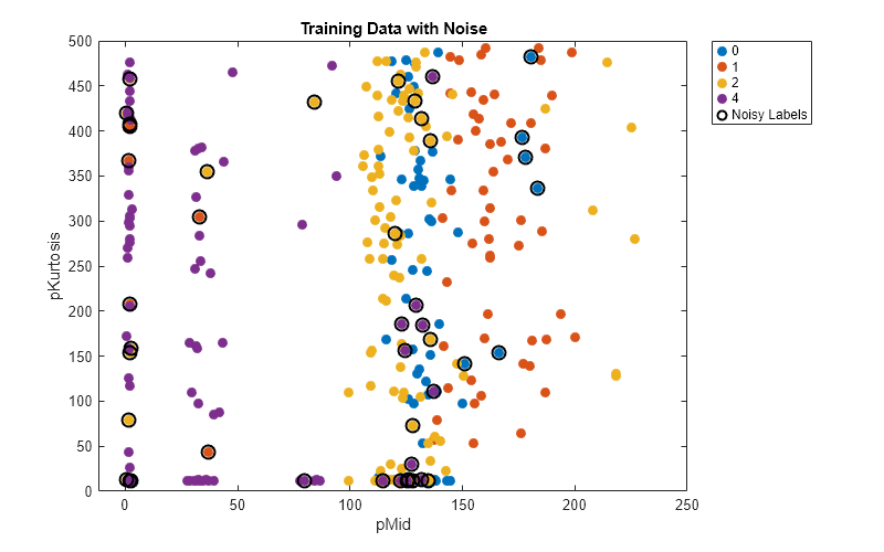
Out of the 353 observations in the training data, 46 have noisy labels in noisyTrainingLabels. That is, these observations are mislabeled due to the added noise.
Visualize Results
Plot the training data so that each point corresponds to an observation, and the color of the point corresponds to the observation label in noisyTrainingLabels. Circle in black the observations with noisy labels.
variableNames = trainingData.Properties.VariableNames; variable1 =variableNames(3); variable2 =
variableNames(5); figure(Position=[1000 800 800 500]) gscatter(trainingData{:,variable1},trainingData{:,variable2}, ... noisyTrainingLabels,[],[],20) hold on scatter(trainingData{trueIssues,variable1},trainingData{trueIssues,variable2}, ... 80,"black",LineWidth=1.5) hold off title("Training Data with Noise") xlabel(variable1) ylabel(variable2) ll = legend(Location="northeastoutside"); ll.String{5} = "Noisy Labels";

In this example, the observation with a pMid value of 1.6 and a pKurtosis value of 79.5 has the incorrect label 2 in noisyTrainingLabels.
Train Model on Noisy Data and Compute Test Loss
Train an ensemble classifier on the training data with noisy labels. Use a bagged ensemble of 200 trees, and specify the order of the labels.
rng(0,"twister") % For reproducibility
labelNames = unique(trueTrainingLabels);
mdlNoisy = fitcensemble(trainingData,noisyTrainingLabels,Method="Bag", ...
    NumLearningCycles=200,ClassNames=labelNames);
Evaluate the performance of the model on the test set by computing the rate of misclassified observations.
lossNoisy = loss(mdlNoisy,testData,trueTestLabels)
lossNoisy =
0.1138
The model accurately predicts the label for approximately 89% of the observations in the test set.
Identify and Prune Noisy Labels
Identify and prune the noisy labels in noisyTrainingLabels. First, generate cross-validated predicted probabilities for the training observations. Then, compute the confident joint matrix to identify label errors. Finally, rank the label errors and determine which observations to remove from the training data set.
Generate Cross-Validated Predicted Probabilities
Cross-validate a classifier that returns predicted probabilities for the observations with the labels noisyTrainingLabels. In this example, use the same type of model as mdlNoisy. In general, you can use a different model, such as the cross-validated tree model returned by fitctree(trainingData,noisyTrainingLabels,KFold=10).
rng(0,"twister")
cvmdl = crossval(mdlNoisy,KFold=10);
Compute the cross-validated predicted probabilities.
[~,predProbs] = kfoldPredict(cvmdl);
predProbs(i,j) indicates the probability that observation i has label j, according to the model cvmdl.
Compute Confident Joint and Identify Label Errors
Use the helper function helperIdentifyLabelIssues to compute the confident joint for the observations with the labels noisyTrainingLabels and the predicted probabilities predProbs. The confident joint is a matrix that estimates the number of correct labels and label errors among the confidently labeled observations. Each row corresponds to an observed label, and each column corresponds to a true label. The off-diagonal entries indicate the number of label errors.
[labelIssueMask,confidentJoint] = helperIdentifyLabelIssues( ...
    noisyTrainingLabels,predProbs);
confidentJointDisplay = array2table(confidentJoint, ...
    VariableNames="TrueLabel=" + string(labelNames), ...
    RowNames="ObservedLabel=" + string(labelNames))
confidentJointDisplay=4×4 table
                       TrueLabel=0    TrueLabel=1    TrueLabel=2    TrueLabel=4
                       ___________    ___________    ___________    ___________

    ObservedLabel=0        54              6              2              0
    ObservedLabel=1         0             41              0              7
    ObservedLabel=2        19              0             59              7
    ObservedLabel=4         6              0              1             56
Of the labels in noisyTrainingLabels, the confident joint considers 48 (6+2+7+19+7+6+1) to be label errors. These labels have a value of 1 (true) in labelIssueMask.
Note that confidentJoint includes counts only for observations where the true label is confidently predicted (that is, the predicted probability for at least one of the labels is greater than or equal to the average for that label). Therefore, confidentJoint might not include counts for observations where the predicted probabilities are low across all labels. As a result, the sum of the entries of confidentJoint can be less than the number of observations.
Use the helper function helperCalibrateConfidentJoint to calibrate confidentJoint so that the sum of the entries matches the total number of labels in noisyTrainingLabels.
calibratedCJ = helperCalibrateConfidentJoint(confidentJoint,noisyTrainingLabels);
labelNames = unique(noisyTrainingLabels);
calibratedCJDisplay = array2table(calibratedCJ, ...
    VariableNames="TrueLabel=" + string(labelNames), ...
    RowNames="ObservedLabel=" + string(labelNames))
calibratedCJDisplay=4×4 table
                       TrueLabel=0    TrueLabel=1    TrueLabel=2    TrueLabel=4
                       ___________    ___________    ___________    ___________

    ObservedLabel=0        80              9              3              0
    ObservedLabel=1         0             54              0              9
    ObservedLabel=2        25              0             77              9
    ObservedLabel=4         8              0              2             77
The calibrated confident joint is useful for retraining the model with observation weights after removing observations with noisy labels from the training data.
Rank Label Errors
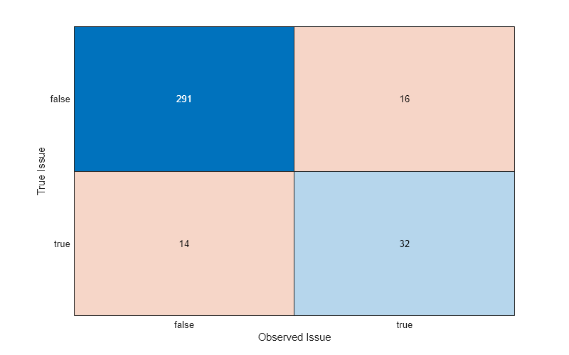
Recall that labelIssueMask indicates the label errors found by the confident joint. In this example, the true label errors are known, and trueIssues indicates which observations truly have noisy labels. Compare the two sets of observations.
confusionchart(trueIssues,labelIssueMask)
xlabel("Observed Issue")
ylabel("True Issue")

Of the 46 true issues (that is, observations that truly have noisy labels), the confident joint correctly identifies 32 issues.
To rank the label errors, first use the helper function helperComputeNormalizedMargin to compute the normalized margin for each observation. A value close to 1 indicates that the observation has a label that is likely correct. A value close to 0 indicates that the observation has a label that is likely incorrect.
normalizedMargin = helperComputeNormalizedMargin(noisyTrainingLabels,predProbs);
Rank the observations identified as having label errors, based on the normalizedMargin values.
labelIssueIndices = find(labelIssueMask);
labelQualityScores = normalizedMargin(labelIssueIndices);
[sortedScores,sortIndices] = sort(labelQualityScores,"ascend");
labelIssueIndicesSortedByScores = labelIssueIndices(sortIndices);
sortedScores contains the normalized margins for the observed issues, sorted from lowest to highest.
Create Report Table
Display the results in a table. For each observed issue, include the index of the observation in the training data, the normalized margin score, and the observed label in noisyTrainingLabels. In this example, include the true label in trueTrainingLabels and the true issue logical value in trueIssues. The true label and true issue values are not known in real data sets and are included here for illustrative purposes only.
issueReport = table(labelIssueIndicesSortedByScores,sortedScores, ...
    noisyTrainingLabels(labelIssueIndicesSortedByScores), ...
    trueTrainingLabels(labelIssueIndicesSortedByScores), ...
    trueIssues(labelIssueIndicesSortedByScores), ...
    VariableNames=["Observation Index","Score","Observed Label", ...
    "True Label*","True Issue*"])
issueReport=48×5 table
    Observation Index    Score     Observed Label    True Label*    True Issue*
    _________________    ______    ______________    ___________    ___________

           286                0          0                1            true
            64            0.005          0                1            true
            10            0.015          0                1            true
            31           0.0225          0                1            true
           242            0.025          0                1            true
           306           0.0275          2                4            true
             6             0.05          0                1            true
           129             0.06          2                2            false
           277             0.08          2                4            true
           221            0.105          1                4            true
           191            0.105          2                4            true
           334             0.11          2                4            true
           181            0.115          1                4            true
           161           0.1325          2                4            true
           272           0.1325          4                0            true
           207           0.1525          1                4            true
      ⋮
The first 20 label errors, as ranked by the normalized margin, are all true issues except for one (label 129).
Visualize Results
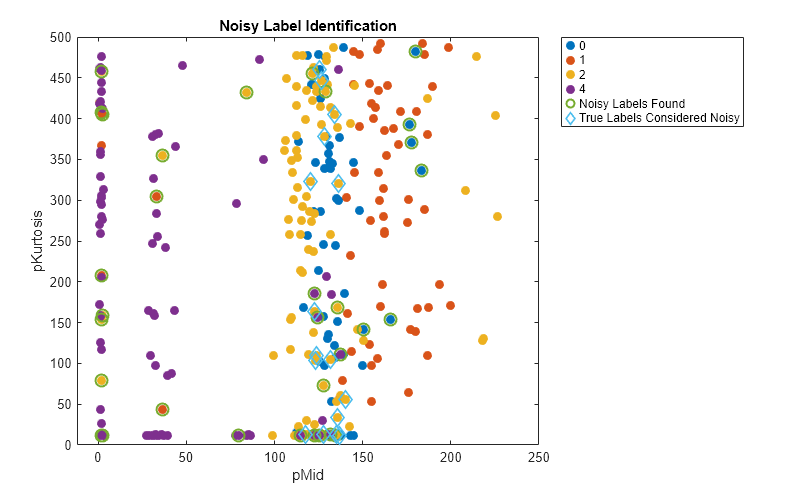
Plot the training data again. In this case, circle in green the observations with noisy labels in noisyTrainingLabels that are correctly identified as label errors. Use light blue diamonds to mark the observations that are incorrectly identified as mislabeled.
variable1 =variableNames(3); variable2 =
variableNames(5); trueIssueIndices = find(trueIssues); issuesFoundTrue = ismember(labelIssueIndices,trueIssueIndices); figure(Position=[1000 800 800 500]) gscatter(trainingData{:,variable1},trainingData{:,variable2}, ... noisyTrainingLabels,[],[],20) hold on scatter(trainingData{labelIssueIndices(issuesFoundTrue),variable1}, ... trainingData{labelIssueIndices(issuesFoundTrue),variable2},80, ... LineWidth=1.5) scatter(trainingData{labelIssueIndices(~issuesFoundTrue),variable1}, ... trainingData{labelIssueIndices(~issuesFoundTrue),variable2},80, ... "diamond",LineWidth=1.5) hold off title("Noisy Label Identification") xlabel(variable1); ylabel(variable2); ll = legend(Location="northeastoutside"); ll.String{5} = "Noisy Labels Found"; ll.String{6} = "True Labels Considered Noisy";

In this example, the observation with a pMid value of 1.6 and a pKurtosis value of 79.5 is correctly identified as mislabeled.
Train Model with Noisy Data Removed and Compute Test Loss
Remove the observations identified as having noisy labels from the training data.
XClean = trainingData(~labelIssueMask,:);
YClean = noisyTrainingLabels(~labelIssueMask,:);
Reweight the training observations using the calibrated confident joint to account for the removed observations.
noiseMatrixComputed = calibratedCJ./sum(calibratedCJ);
weightsPerClass = 1./diag(noiseMatrixComputed);
weights = zeros(size(YClean));
for i = 1:numel(labelNames)
    idxClasses = YClean == labelNames(i);
    weights(idxClasses) = weightsPerClass(i);
end
Retrain the ensemble classifier with the cleaned training data and the computed observation weights. Use the same model specifications as mdlNoisy.
rng(0,"twister")
mdlCleaned = fitcensemble(XClean,YClean,Weights=weights, ...
    Method="Bag",NumLearningCycles=200,ClassNames=labelNames);
In this example, compute the test set loss for mdlCleaned and compare it to the previously computed loss for mdlNoisy.
lossCleaned = loss(mdlCleaned,testData,trueTestLabels)
lossCleaned =
0.0975
lossNoisy
lossNoisy =
0.1138
The mdlCleaned model accurately predicts the label for approximately 90% of the observations in the test set, which is better than the accuracy of the mdlNoisy model.
Helper Functions
helperGenerateNoisyLabels
The helperGenerateNoisyLabels function takes a vector of true labels (truelabels) and applies noise to the labels based on the specified K-by-K noise rate matrix (noiseRate), where K is the number of unique labels. The rows and columns of the noise rate matrix must be in the order of unique(truelabels). The function returns the noisy labels (noisyLabels).
function noisyLabels = helperGenerateNoisyLabels(truelabels,noiseRate)

labels = unique(truelabels);
K = numel(labels);

[counts,~] = groupcounts(truelabels(:));
py = counts./sum(counts);

jointCount = int32(noiseRate.*py'*numel(truelabels));
diags = logical(eye(K));
jointCount(diags) = 0; % Diagonal entries are not flipped

noisyLabels = truelabels;
for ij = 1:K
    idxfliptolabels = jointCount(:,ij) ~= 0;
    fliptolabels = labels(idxfliptolabels);
    numfliptolabels = jointCount(idxfliptolabels,ij);
    noise = repelem(fliptolabels,numfliptolabels');

    idxcanflip = find(truelabels == labels(ij));
    subsetIdx = randperm(numel(idxcanflip),sum(numfliptolabels));
    idxtoflip = idxcanflip(subsetIdx);

    noisyLabels(idxtoflip) = noise;
end
end
helperIdentifyLabelIssues
The helperIdentifyLabelIssues function takes noisyTrainingLabels, a vector of noisy labels of length n with one label for each observation, and predProbs, a matrix of predicted probabilities of size n-by-K, where K is the number of unique labels. The columns of the predicted probabilities matrix must be in the order of unique(noisyTrainingLabels).
The function computes the confident joint (confidentJoint), a K-by-K matrix, using these steps:
For each unique label, the function determines the average predicted probability (average self-confidence).
For each observation, the function determines whether the predicted probability for at least one of the labels is greater than or equal to the average for that label. If so, the function counts the observation in the confident joint entry
confidentJoint(i,j), whereiis the observed label andjis the label with the greatest predicted probability. Otherwise, the function does not include the observation in theconfidentJointcomputation.
The function additionally returns labelIssueMask, a logical vector of length n. A value of 1 (true) indicates that the corresponding observation has a label error in noisyTrainingLabels.
function [labelIssueMask,confidentJoint] = helperIdentifyLabelIssues( ...
    noisyTrainingLabels,predProbs)

    classNames = unique(noisyTrainingLabels);
    K = numel(classNames);
    N = numel(noisyTrainingLabels);

    % Compute the thresholds
    thresholds = nan(1,K);
    C = false(N,K);
    % Get labels to index in the K columns in order of mdl.ClassNames
    catNoisyLabels = categorical(noisyTrainingLabels,classNames);
    idxNoisyLabels = grp2idx(catNoisyLabels);
    idx = sub2ind([N K],(1:N)',idxNoisyLabels); % Row and column to index
    C(idx) = true;
    for ij = 1:K
        thresholds(ij) = mean(predProbs(C(:,ij),ij));
    end

    % Compute the confident joint while handling label collisions
    predProbBool = predProbs >= thresholds - 1e-6;
    numConfidentBins = sum(predProbBool,2);
    atLeastOneConfident = numConfidentBins > 0;
    moreThanOneConfident = numConfidentBins > 1;

    % For each observation, choose the confident class (greater than threshold)
    % as trueLabelIndexGuess
    [~,confidentArgmax] = max(predProbBool,[],2);
    trueLabelIndexGuess = confidentArgmax;
    % When there are 2+ confident classes, choose the class with the largest probability
    [~,predProbArgmax] = max(predProbs,[],2);
    trueLabelIndexGuess(moreThanOneConfident) = predProbArgmax(moreThanOneConfident);
    % Omit "all false" rows from trueLabelIndexGuess and idxNoisyLabels
    trueLabelIndexGuess = trueLabelIndexGuess(atLeastOneConfident);
    noisyLabelIndexObserved = idxNoisyLabels(atLeastOneConfident);
    % Compute the joint matrix P(noisyLabel,trueLabel)
    confidentJoint = confusionmat(noisyLabelIndexObserved,trueLabelIndexGuess, ...
        Order=1:K);
    % Guarantee that at least one correctly labeled example is represented in every class
    confidentJoint(logical(eye(size(confidentJoint)))) = max(1,diag(confidentJoint));

    % Return the observations in the off-diagonals of the confident joint.
    % These are the observations that are confidently predicted to be a
    % different label from their given label.
    labelsMismatch = trueLabelIndexGuess ~= noisyLabelIndexObserved;
    offDiagnoalIndices = 1:numel(noisyTrainingLabels);
    offDiagnoalIndices = offDiagnoalIndices(atLeastOneConfident);
    offDiagnoalIndices = offDiagnoalIndices(labelsMismatch)';
    labelIssueMask = false(N,1);
    labelIssueMask(offDiagnoalIndices) = true;
end
helperCalibrateConfidentJoint
The helperCalibrateConfidentJoint function takes a confident joint K-by-K matrix (confidentJoint) and a length-n vector of labels (noisyTrainingLabels), where K is the number of unique labels. The function returns the calibrated confident joint confidentJointIntegers, a K-by-K matrix whose entries sum to n.
function confidentJointIntegers = helperCalibrateConfidentJoint( ...
    confidentJoint,noisyTrainingLabels)

classNames = unique(noisyTrainingLabels);
K = numel(classNames);

% Update to maintain prior probability for noisy labels
[counts,~] = groupcounts(noisyTrainingLabels(:));
confidentJointNum = (confidentJoint./sum(confidentJoint,2)).*counts;
% The confident joint should sum to the total number of observations
Qij = confidentJointNum./sum(confidentJointNum(:)); % Estimated joint probability distribution
confidentJointCalibrated = Qij * sum(counts);
% Convert the confident joint to integer values while preserving the row sum
confidentJointIntegers = floor(confidentJointCalibrated);
numAdjustments = counts - sum(confidentJointIntegers,2);
for ij = 1:K
    [~,indices] = sort(confidentJointCalibrated(ij,:) - ...
        confidentJointIntegers(ij,:),"descend");
    confidentJointIntegers(ij,indices(1:numAdjustments(ij))) = ...
        confidentJointIntegers(ij,indices(1:numAdjustments(ij))) + 1;
end
end
helperComputeNormalizedMargin
The helperComputeNormalizedMargin function takes noisyTrainingLabels, a vector of noisy labels of length n with one label for each observation, and predProbs, a matrix of predicted probabilities of size n-by-K, where K is the number of unique labels. The columns of the predicted probabilities matrix must be in the order of unique(noisyTrainingLabels).
The function computes the normalized margin for each observation in the following way:
Determine the predicted probability p in
predProbsfor the observation label innoisyTrainingLabels.Find the maximum predicted probability among the remaining labels pmax.
Take the difference between p and pmax. To keep the normalized margin in the range [0,1], add 1 to the value, and then divide the result by 2.
The returned normalizedMargin is a numeric vector of length n.
function normalizedMargin = helperComputeNormalizedMargin(noisyTrainingLabels,predProbs)
classNames = unique(noisyTrainingLabels);
K = numel(classNames);
N = numel(noisyTrainingLabels);
predProbsT = predProbs';

C = false(N,K);
% Get labels to index in the K columns in order of mdl.ClassNames
catNoisyLabels = categorical(noisyTrainingLabels,classNames);
idxNoisyLabels = grp2idx(catNoisyLabels);
idx = sub2ind([N K],(1:N)',idxNoisyLabels); % Row and column to index
C(idx) = true;

selfConfidence = predProbsT(C');
predProbOfOtherLabels = predProbsT(~C');
predProbOfOtherLabels = reshape(predProbOfOtherLabels,[K-1 N])';
normalizedMargin = ...
    (selfConfidence - max(predProbOfOtherLabels,[],2) + 1)/2; % Results in range [0,1]
end
References
[1] Northcutt, Curtis, Lu Jiang, and Isaac Chuang. "Confident Learning: Estimating Uncertainty in Dataset Labels." Journal of Artificial Intelligence Research 70 (2021): 1373-1411.
See Also
fitcensemble | loss | crossval
Topics
- Multi-Class Fault Detection Using Simulated Data (Predictive Maintenance Toolbox)