fit
Description
The fit function fits a configured model for incremental
k-means clustering (incrementalKMeans
object) to streaming data.
To fit a k-means clustering model to an entire batch of data at once,
use kmeans.
Mdl = fit(Mdl,X)Mdl, which is the
input incrementalKMeans
model object Mdl fit using the predictor data X. Specifically, the
incremental fit function fits the model to the incoming data
and stores the updated clustering properties in the output model Mdl. For more
information, see Incremental k-Means Clustering.
Examples
Create an incremental model for k-means clustering that has two clusters.
Mdl = incrementalKMeans(numClusters=2)
Mdl =
  incrementalKMeans

         IsWarm: 0
        Metrics: [1×2 table]
    NumClusters: 2
      Centroids: [2×0 double]
       Distance: "sqeuclidean"


  Properties, Methods
Mdl is an incrementalKMeans model object. All its properties are read-only.
Load and Preprocess Data
Load the New York city housing data set.
load NYCHousing2015.matThe data set includes 10 variables with information on the sales of properties in New York City in 2015. Keep only the gross square footage and sale price predictors. Keep all records that have a gross square footage above 100 square feet and a sales price above $1000.
data = NYCHousing2015(:,{'GROSSSQUAREFEET','SALEPRICE'});
data = data((data.GROSSSQUAREFEET > 100 & data.SALEPRICE > 1000),:);
Convert the tabular data into a matrix that contains the logarithm of both predictors.
X = table2array(log10(data));
Randomly shuffle the order of the records.
 rng(0,"twister"); % For reproducibility
 X = X(randperm(size(X,1)),:);
Fit and Plot Incremental Model
Fit the incremental model Mdl to the data by using the fit function. To simulate a data stream, fit the model in chunks of 500 records at a time. At each iteration:
Process 500 observations.
Overwrite the previous incremental model with a new one fitted to the incoming records.
Update the performance metrics for the model. The default metric for
MdlisSimplifiedSilhouette.Store the cumulative and window metrics to see how they evolve during incremental learning.
Compute the cluster assignments of all records seen so far, according to the current model.
Plot all records seen so far, and color each record by its cluster assignment.
Plot the current centroid location of each cluster.
In this workflow, the updateMetrics function provides information about the model's clustering performance after it is fit to the incoming data chunk. In other workflows, you might want to evaluate a clustering model's performance on unseen data. In such cases, you can call updateMetrics prior to calling the incremental fit function.
% Initialize plot properties
hold on
h1 = scatter(NaN,NaN,0.3);
h2 = plot(NaN,NaN,Marker="o", ...
    MarkerFaceColor="k",MarkerEdgeColor="k");
h3 = plot(NaN,NaN,Marker="^", ...
    MarkerFaceColor="b",MarkerEdgeColor="b");
colormap(gca,"prism")
pbaspect([1,1,1])
xlim([min(X(:,1)),max(X(:,1))]);
ylim([min(X(:,2)),max(X(:,2))]);
xlabel("log Gross Square Footage");
ylabel("log Sales Price in Dollars")

% Incremental fitting and plotting
n = numel(X(:,1));
numObsPerChunk = 500;
nchunk = floor(n/numObsPerChunk);
sil = array2table(zeros(nchunk,2),VariableNames=["Cumulative" "Window"]);

for j = 1:nchunk
    ibegin = min(n,numObsPerChunk*(j-1) + 1);
    iend = min(n,numObsPerChunk*j);
    idx = ibegin:iend;
    Mdl = fit(Mdl,X(idx,:));
    Mdl = updateMetrics(Mdl,X(idx,:));
    sil{j,:} = Mdl.Metrics{'SimplifiedSilhouette',:};
    indices = assignClusters(Mdl,X(1:iend,:));
    title("Iteration " + num2str(j))
    set(h1,XData=X(1:iend,1),YData=X(1:iend,2),CData=indices);
    set(h2,Marker="none") % Erase previous centroid markers
    set(h3,Marker="none")
    set(h2,XData=Mdl.Centroids(1,1),YData=Mdl.Centroids(1,2),Marker="o")
    set(h3,Xdata=Mdl.Centroids(2,1),YData=Mdl.Centroids(2,2),Marker="^")
    pause(0.5);
end
Warning: Hardware-accelerated graphics is unavailable. Displaying fewer markers to preserve interactivity.
hold off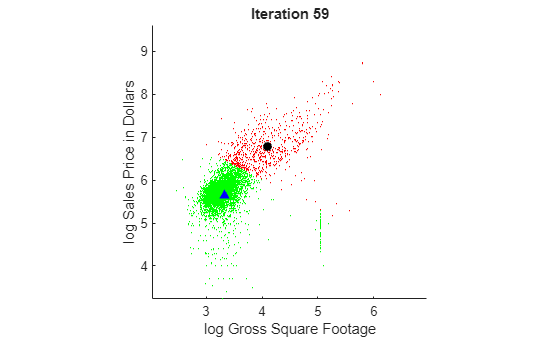
To view the animated figure, you can run the example, or open the animated gif below in your web browser.

At each iteration, the animated plot displays all the observations processed so far as small circles, and colors them according to the cluster assignments of the current model. The black circle indicates the centroid position of cluster 1, and the blue triangle indicates the centroid position of cluster 2.
Plot the window and cumulative metrics values at each iteration.
h4 = plot(sil.Variables);
xlabel("Iteration")
ylabel("Performance Metric")
xline(Mdl.WarmupPeriod/numObsPerChunk,'g-.')
legend(h4,sil.Properties.VariableNames,Location="southeast")
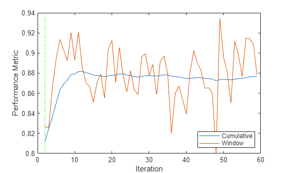
The updateMetrics function calculates the performance metrics after the end of the warm-up period. The performance metrics rise rapidly from an initial value of 0.81 and approach a value of approximately 0.88 after 10 iterations.
Create a set of noisy position measurements of two moving objects. Object 1 starts at (x,y) coordinate (-50,0) and moves along the x-axis. Object 2 starts at (x,y) coordinate (0,-40) and moves along the y-axis. The objects move at the same speed.
Generate numObsPerStep=100 measurements of each object at numSteps=100 individual time steps.
rng(0,"twister") % For reproducibility
sigma = 2;  % Measurement noise level
numObsPerStep = 100;
numSteps = 100;
startPosA = [-50,0];
startPosB = [0,-40];
X = [];
for t = 0:numSteps-1
    for i = 1:numObsPerStep
        p = randn(1,4)*sigma;  % Gaussian measurement noise
        X = [X;[[p(1)+t+startPosA(1);p(2)+startPosB(1)], ...
            [p(3)+startPosA(2);p(4)+t+startPosB(2)]]];
    end
end
The rows of X contain 2*numObsPerStep*numSteps position measurements. The columns of X contain the x and y coordinates of each measurement, respectively.
Create Incremental k-Means Clustering Models
To track the centroids of the moving clusters, create two incremental k-means clustering model objects that each have two clusters and no warm-up period. Specify a forgetting factor value of 0.1 for the first model, and 0.75 for the second model. A lower value of the forgetting factor (which can range from 0 to 1) assigns more weight to older measurements when the incremental fit algorithm calculates new cluster centroids.
MdlA = incrementalKMeans(numClusters=2,WarmupPeriod=0, ...
    ForgettingFactor=0.1);
MdlB = incrementalKMeans(numClusters=2,WarmupPeriod=0, ...
    ForgettingFactor=0.75);
Fit and Plot Incremental Models
Fit the incremental k-means clustering models to the data by using the fit function. Fit the models in data chunks that consist of the measurements at each time step. At each iteration:
Process
2*numObsPerStepobservations.Overwrite the previous incremental models with new ones fitted to the incoming measurements.
Update the performance metrics for the models. The metric for the models is
SimplifiedSilhouette.Store the cumulative and window metrics to see how they evolve during incremental learning.
Compute the cluster assignments of the incoming chunk of measurements, according to the current model A.
Plot the incoming chunk of measurements, and color each measurement by its cluster assignment according to model A.
Plot the current model centroid locations for each cluster.
Plot all of the previous measurements using gray points.
% Initialize plot properties
hold on
h1 = scatter(NaN,NaN,0.2,[0.9 0.9 0.9],".");
h2 = scatter(NaN,NaN,1.5);
h3 = plot(NaN,NaN,"^",MarkerSize=6,MarkerEdgeColor="k", ...
    MarkerFaceColor="k");
h4 = plot(NaN,NaN,"square",MarkerSize=6,MarkerEdgeColor="b", ...
    MarkerFaceColor="b");
colormap(gca,"prism")
xlim([min(X(:,1)),max(X(:,1))]);
ylim([min(X(:,2)),max(X(:,2))]);
xlabel("X");
ylabel("Y");
% Incremental fitting and plotting
n = numel(X(:,1));
nChunk = 2*numObsPerStep;
silA = array2table(zeros(numSteps,2), ...
    'VariableNames',["Cumulative" "Window"]);
silB = array2table(zeros(numSteps,2), ...
    'VariableNames',["Cumulative" "Window"]);
for j = 1:numSteps
    ibegin = min(n,nChunk*(j-1) + 1);
    iend = min(n,nChunk*j);
    idx = ibegin:iend;
    [MdlA,indices] = fit(MdlA,X(idx,:));
    MdlA = updateMetrics(MdlA,X(idx,:));
    MdlB = fit(MdlB,X(idx,:));
    MdlB = updateMetrics(MdlB,X(idx,:));
    title("Iteration " + num2str(j))
    silA{j,:} = MdlA.Metrics{'SimplifiedSilhouette',:};
    silB{j,:} = MdlB.Metrics{'SimplifiedSilhouette',:};
    set(h1,XData=X(1:ibegin-1,1),YData=X(1:ibegin-1,2));
    set(h2,XData=X(idx,1),YData=X(idx,2),CData=indices);
    set(h3,Marker="none") % Erase the previous centroid markers
    set(h4,Marker="none")
    set(h3,XData=MdlA.Centroids(:,1),YData=MdlA.Centroids(:,2), ...
        Marker="^");
    set(h4,XData=MdlB.Centroids(:,1),YData=MdlB.Centroids(:,2), ...
        Marker="square");
    pause(0.2);
end
hold off
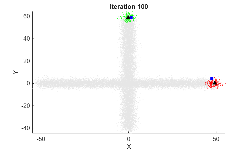
 At each iteration, the animated plot displays all of the position measurements processed so far in gray. The incremental
 fit function tracks the centroid of each object at each iteration. The measurements in the current data chunk are colored according to the cluster assignment of model A. The black upward-pointing triangles and blue squares indicate the fitted cluster centroids of models A and B, respectively.
Model A does a good job of tracking the true position of each moving object. Because model B has a higher forgetting factor, the fit function assigns the highest weights to the most recent measurements. Therefore, model B does a poorer job of tracking the true positions of the objects.
Plot the simplified silhouette performance metrics at each iteration.
h5 = plot([silA.Variables,silB.Variables]);
xlabel("Iteration")
ylabel("Simplified Silhouette")
legend(h5,{"Cumulative A","Window A", ...
    "Cumulative B","Window B"},Location="southwest")
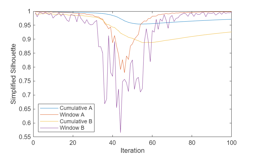
The plot shows that the simplified silhouette values of model B are poorer than those of model A. The values of both models dip significantly between iterations 30 and 60, when the two objects are close to each other. As the objects move apart, the window values of both models return to their previous levels.
Input Arguments
Output Arguments
More About
References
[1] Lloyd, S. Least Squares Quantization in PCM. IEEE Transactions on Information Theory 28, no. 2 (March 1982): 129–37.
[2] Sculley, D. Web-Scale k-Means Clustering. In Proceedings of the 19th International Conference on World Wide Web, 1177–78. Raleigh North Carolina USA: ACM, 2010.
Version History
Introduced in R2025a