mdscale

Nonclassical multidimensional scaling

Syntax

Y = mdscale(D,p)

Y = mdscale(___,Name=Value)

[Y,stress]= mdscale(___)

[Y,stress,disparities]= mdscale(___)

Description

Y = mdscale(D,p) performs nonmetric multidimensional scaling on the n-by-n dissimilarity matrix D, and returns an n-by-p configuration matrix. The rows of Y correspond to the coordinates of n points in p-dimensional space. The Euclidean distances between the points in Y approximate a monotonic transformation of the corresponding dissimilarities in D. By default, mdscale uses Kruskal's normalized stress formula 1 criterion. To perform metric multidimensional scaling, specify the Criterion name-value argument.

example

Y = mdscale(___,Name=Value) specifies additional options using one or more name-value arguments. For example, you can specify dissimilarity weights, and the goodness-of-fit criterion to minimize.

example

[Y,stress]= mdscale(___) additionally returns the minimized stress, which is the stress evaluated at Y.

example

[Y,stress,disparities]= mdscale(___) additionally returns the disparities, which are a monotonic transformation of the dissimilarities in D.

example

Examples

collapse all

Perform Multidimensional Scaling

Open Live Script

Perform nonmetric and metric scaling on the same data set.

Load the cereal data set, which contains nutritional information for 77 cereals.

load cereal

Take a subset of the data that consists of selected measurements of cereals from a single manufacturer.

X = [Calories,Protein,Fat,Sodium,Fiber, ...
    Carbo,Sugars,Shelf,Potass,Vitamins];
X = X(strcmp("K",cellstr(Mfg)),:);
size(X)

ans = 1×2

    23    10

X contains 23 observations and 10 predictor variables.

Create a dissimilarity matrix using the pdist function.

dissimilarities = pdist(X)

dissimilarities = 1×253

  122.2784  322.6329  288.6226  347.3615  204.0662  295.9206  322.6050  303.9539  342.0409  141.1241  288.2603  263.6001  214.4808  293.1996  206.9734  248.1290  293.2388  107.3126  334.9910  289.9034  340.9883  269.9685  306.9267  335.2238  320.2312  180.7291  316.7823  306.8843  317.1183  274.2408  186.4457  288.6451  264.9925  203.6566  303.0380  234.1880  245.6135  349.3895  134.7739  264.2593  336.9481  304.9607  295.9307  166.1174   36.5240  131.1297   96.1613    1.4142   75.2994  143.8332

size(squareform(dissimilarities))

ans = 1×2

    23    23

dissimilarities is a row vector that contains the 253 upper triangle elements of the dissimilarity matrix, which has size 23-by-23.

Use nonmetric scaling to recreate the data in two dimensions.

[Y,~,disparities] = mdscale(dissimilarities,2);
distances = pdist(Y);

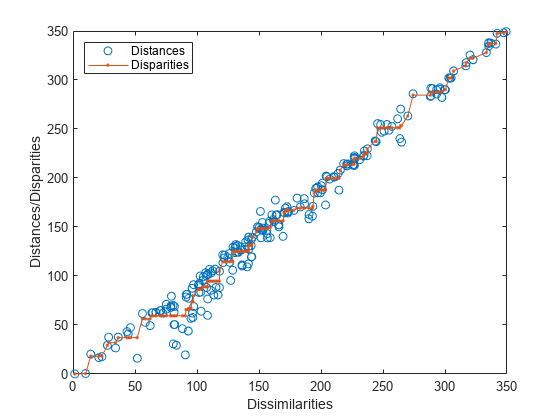
Visualize the results using a Shepard plot.

[~,ord] = sortrows([disparities(:),dissimilarities(:)]);
plot(dissimilarities,distances,"o", ...
    dissimilarities(ord),disparities(ord),".-");
axis square
xlim([0 max(dissimilarities)]);
ylim([0 max(dissimilarities)]);
xlabel("Dissimilarities")
ylabel("Distances/Disparities")
legend(["Distances","Disparities"],Location="northwest");

Figure contains an axes object. The axes object with xlabel Dissimilarities, ylabel Distances/Disparities contains 2 objects of type line. One or more of the lines displays its values using only markers These objects represent Distances, Disparities.

The x coordinates of the blue circles correspond to their original dissimilarity values, and the y coordinates correspond to their Euclidean distances in two-dimensional space. Most points lie close the 1:1 line, indicating that a two-dimensional scaling provides a reasonably good representation of the higher-dimensional dissimilarities. The connected red points indicate the disparity values, which are a monotonic transformation of the dissimilarities.

Perform metric scaling on the same dissimilarities using the metricsstress criterion.

[Y,stress] = mdscale(dissimilarities,2,Criterion="metricsstress");
distances = pdist(Y);

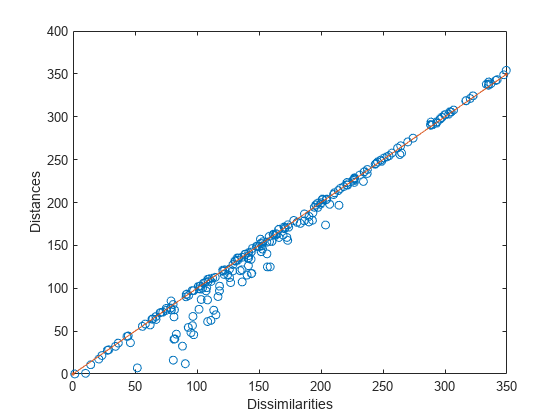
Visualize the results using a Shepard plot. Because there are no dissimilarities in metric scaling, plot a red 1:1 line.

plot(dissimilarities,distances,"o", ...
    [0 max(dissimilarities)],[0 max(dissimilarities)],".-")
%xlim([0 max(dissimilarities)]);
axis square;
xlim([0 max(dissimilarities)]);
ylim([0 max(dissimilarities)]);
xlabel("Dissimilarities")
ylabel("Distances")

Figure contains an axes object. The axes object with xlabel Dissimilarities, ylabel Distances contains 2 objects of type line. One or more of the lines displays its values using only markers

Most points lie very close to the 1:1 line, indicating that a two-dimensional metric scaling provides a good representation of the higher-dimension dissimilarities.

Nonmetric Multidimensional Scaling

Open Live Script

This example shows how to perform nonmetric multidimensional scaling using mdscale .

Metric multidimensional scaling (MDS) creates a configuration of points whose interpoint distances approximate the given dissimilarities. This is sometimes too strict a requirement, and nonmetric scaling provides a less strict alternative. Instead of trying to approximate the dissimilarities themselves, nonmetric scaling approximates a nonlinear, but monotonic, transformation of them. Because of the monotonicity, larger or smaller distances on a plot of the output will correspond to larger or smaller dissimilarities, respectively. However, the nonlinearity implies that mdscale only attempts to preserve the ordering of dissimilarities. Thus, there may be contractions or expansions of distances at different scales.

Load the cereal data set, which contains measurements of 10 variables describing 77 breakfast cereals.

rng(0,"twister"); % For reproducibility
load cereal

Take a subset of the data that consists of selected measurements of cereals from a single manufacturer.

X = [Calories Protein Fat Sodium Fiber ... 
    Carbo Sugars Shelf Potass Vitamins];
X = X(strcmp("G",cellstr(Mfg)),:);
size(X)

ans = 1×2

    22    10

X contains 22 observations and 10 predictor variables.

Use pdist to transform the 10-dimensional data into dissimilarities. First standardize the cereal data, and use city block distance as a dissimilarity.

dissimilarities = pdist(zscore(X),'cityblock');
size(dissimilarities)

ans = 1×2

     1   231

The output from pdist is a symmetric dissimilarity matrix, stored as a vector containing only the (22*21/2) elements in its upper triangle. The choice of transformation to dissimilarities is application-dependent, and is made here only for simplicity. In some applications, the original data is already in the form of dissimilarities.

Use mdscale to perform nonmetric multidimensional scaling with Kruskal's stress formula 1 model .

[Y,stress,disparities] = mdscale(dissimilarities,2,Criterion="stress");
stress

stress = 
0.1562

The nonmetric stress criterion is a common method for computing the output; for more choices, see the mdscale reference page in the online documentation. The second output from mdscale is the value of that criterion evaluated for the output configuration. It is a measure of how well the inter-point distances of the output configuration approximate the disparities. The disparities are returned in the third output. They are the monotonically transformed values of the original dissimilarities.

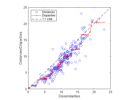
Visualize these data to check the fit of the output configuration to the dissimilarities and to understand the disparities.

distances = pdist(Y);
[dum,ord] = sortrows([disparities(:) dissimilarities(:)]);
plot(dissimilarities,distances,"bo",dissimilarities(ord),...
     disparities(ord),"r.-",[0 25],[0 25],"k--")
axis square;
xlabel("Dissimilarities")
ylabel("Distances/Disparities")
legend({"Distances" "Disparities" "1:1 Line"},...
       "Location","NorthWest");

Figure contains an axes object. The axes object with xlabel Dissimilarities, ylabel Distances/Disparities contains 3 objects of type line. One or more of the lines displays its values using only markers These objects represent Distances, Disparities, 1:1 Line.

mdscale finds a configuration of points in two dimensions whose inter-point distances approximates the disparities, which in turn are a nonlinear transformation of the original dissimilarities. The concave shape of the disparities as a function of the dissimilarities indicates that fit tends to contract small distances relative to the corresponding dissimilarities. This might be perfectly acceptable in practice.

mdscale uses an iterative algorithm to find the output configuration, and the results can often depend on the starting point. By default, mdscale uses cmdscale to construct an initial configuration, and this choice often leads to a globally best solution. However, it is possible for mdscale to return a configuration that is a local minimum of the criterion. Such cases can be diagnosed and often overcome by running mdscale multiple times with different starting points. You can do this using the Start and Replicates name-value arguments.

Repeat the scaling, this time using five replicates of MDS, each starting at a different randomly-chosen initial configuration. mdscale displays a final stress criterion for each replication, and returns the configuration with the best fit.

[Y,stress] = mdscale(dissimilarities,2,Criterion="stress",...  
         Start="random",Replicates=5, ...
         Options=statset(Display="final"));

35 iterations, Final stress criterion = 0.156209
31 iterations, Final stress criterion = 0.156209
48 iterations, Final stress criterion = 0.171209
33 iterations, Final stress criterion = 0.175341
32 iterations, Final stress criterion = 0.185881

Notice that mdscale finds several different local solutions, some of which do not have as low a stress value as the solution found with the cmdscale starting point.

Input Arguments

collapse all

`D` — Dissimilarity matrix
`n`-by-`n` numeric matrix | 1-by-`k` numeric vector

Dissimilarity matrix for n points, specified as an n-by-n numeric matrix. You can also specify D as a 1-by-k numeric vector that contains the n*(n-1)/2 upper triangle elements of the dissimilarity matrix. In this case, the software converts D into a square matrix using the squareform function. The software treats NaNs as missing values and ignores them. D cannot contain any negative or Inf values, and must be one of the following matrix types:

Matrix Type	Symmetric	Description
Full dissimilarity	Yes	Zeros along the diagonal, and nonnegative dissimilarity values off the diagonal
Full dissimilarity (upper triangle form)	No	Nonnegative dissimilarity values above the diagonal, and zeros elsewhere
Full similarity	Yes	Ones along the diagonal, and nonnegative values less than one off the diagonal `mdscale` transforms a similarity matrix to a dissimilarity matrix so that the distances between the points in `Y` equal or approximate `sqrt(1–D)`. To use a different transformation, transform the similarities prior to calling `mdscale`.

Data Types: single | double

`p` — Dimensionality of desired embedding
integer between 1 and `n` | []

Dimensionality of desired embedding, specified as an integer between 1 and n, where n is the number of points in D. If you specify p=[], you must also specify Start as an n-by-k matrix. In this case, the software sets p=k.

Data Types: single | double

Name-Value Arguments

Specify optional pairs of arguments as Name1=Value1,...,NameN=ValueN, where Name is the argument name and Value is the corresponding value. Name-value arguments must appear after other arguments, but the order of the pairs does not matter.

Example: mdscale(D,2,Criterion="sammon")

`Criterion` — Goodness-of-fit criterion
`"stress"` (default) | `"sstress"` | `"metricstress"` | `"metricsstress"` | `"sammon"` | `"strain"`

Goodness-of-fit criterion to minimize, specified as one of the values in the following table. This argument also determines the type of scaling that mdscale performs. In metric scaling, the interpoint distances in Y approximate the dissimilarities in D. In nonmetric scaling, the interpoint distances in Y approximate the disparities, which are a monotonic transformation of the dissimilarities in D.

Value	Scaling Type	Description
`"stress"` (default)	Nonmetric	Stress normalized by the sum of squares of the interpoint distances, also known as Kruskal's stress formula 1 [4]
`"sstress"`	Nonmetric	Squared stress, normalized with the sum of 4th powers of the interpoint distances. This criterion is more sensitive to large discrepancies between points than stress formula 1.
`"metricstress"`	Metric	Stress, normalized with the sum of squares of the dissimilarities
`"metricsstress"`	Metric	Squared stress, normalized with the sum of 4th powers of the dissimilarities
`"sammon"`	Metric	Sammon's nonlinear mapping criterion. Unlike Kruskal's stress formula 1, which treats all distances equally, Sammon's criterion emphasizes the preservation of small distances. This can make the algorithm more computationally intensive and slower to converge [5].
`"strain"`	Metric	A criterion equivalent to that used in classical multidimensional scaling

Example: Criterion="sstress"

Data Types: char | string

`Weights` — Dissimilarity weights
`n`-by-`n` symmetric numeric matrix of nonnegative values | 1-by-`n*(n-1)/2` numeric vector of nonnegative values

Dissimilarity weights, specified as an n-by-n symmetric numeric matrix of nonnegative values, or a 1-by-n*(n-1)/2 numeric vector of nonnegative values, where n is the number of points in D. Weights must have the same size as D. When mdscale computes and minimizes stress, it weighs the elements of D with the corresponding values in Weights. The software effectively ignores any elements of D with a corresponding zero weight value.

Note

When you specify weights as a full matrix, its diagonal elements are ignored and have no effect, since the corresponding diagonal elements of D do not enter into the stress calculation.

Data Types: single | double

`Start` — Method for selecting initial configuration of points
`"cmdscale"` (default) | `"random"` | numeric matrix

Method for selecting initial configuration of points for Y, specified as one of the values in this table.

Value	Description
`"cmdscale"` (default)	The software constructs an initial classical multidimensional scaling configuration using the `cmdscale` function. This value is not valid when you specify `Weights` and at least one weight value is zero.
`"random"`	The software chooses point locations randomly from an appropriately scaled `p`-dimensional normal distribution with uncorrelated coordinates.
numeric matrix	An n-by-`p` matrix of initial locations, where n is the number of points in `D`. In this case, when you specify `p=[]`, the software infers `p` from the second dimension of the matrix. You can also specify `Start` as a 3-D array that contains multiple initial configurations. In this case, if you do not specify `Replicates`, the software sets `Replicates` to the size of the array's third dimension.

Tip

To reduce the likelihood that the software finds only a local minimum solution, try running mdscale multiple times with different starting points, and specify a larger value of Replicates.

Example: Start="random"

Data Types: char | string | single | double

`Replicates` — Number of times to repeat the scaling
`1` (default) | nonnegative integer

Number of times to repeat the scaling, specified as a nonnegative integer. If you do not specify Start, the software sets Replicates=1. If you specify Start as a 3-D array:

Replicates must equal the size of the array's third dimension.
If you do not specify Replicates, the software sets Replicates to the size of the array's third dimension.

At each iteration, mdscale uses a new initial configuration. You can specify this argument to reduce the likelihood that mdscale finds only a local minimum solution.

Example: Replicates=3

Data Types: single | double

`Options` — Options for the iterative fitting criterion minimization algorithm
structure

Options for the iterative fitting criterion minimization algorithm, specified as a structure. Create the Options structure using statset. This table lists the option fields and their values.

Field Name	Value	Default
`Display`	Amount of information to display, specified as one of the following: `"off"` —no information `"iter"` — iteration output `"final"` — final output only	`"off"`
`MaxIter`	Maximum number of iterations, specified as a positive integer.	`200`
`TolFun`	Termination tolerance for the stress criterion and its gradient, specified as a positive scalar value.	`1e-4`
`TolX`	Termination tolerance for the configuration location step size, specified as a positive scalar value.	`1e-4`

Example: Options=statset(Display="final", MaxIter=10)

Data Types: struct

Output Arguments

collapse all

`Y` — Configuration matrix
`n`-by-`p` numeric matrix

Configuration matrix for the n-by-n matrix D, returned as an n-by-p numeric matrix. The rows of Y correspond to the coordinates of n points in p-dimensional space. The software seeks to find a configuration matrix that minimizes the value of stress.

`stress` — Stress
numeric scalar

Stress evaluated at Y, returned as a numeric scalar. For nonmetric scaling (the default), the stress value is a measure of how well the interpoint distances of the output configuration matrix Y approximate the disparities. For metric scaling, the stress value is a measure of how well the interpoint distances of the output configuration matrix approximate the input dissimilarities D.

`disparities` — Disparities
numeric matrix

Disparities, returned as a numeric matrix of the same size as D. For nonmetric scaling, the disparities are the monotonic transformed values of the dissimilarities in D. For metric scaling, there are no disparities, and mdscale returns D.

References

[1] Cox, Trevor F., and Michael A. A. Cox. Multidimensional Scaling. 2nd ed. Monographs on Statistics and Applied Probability 88. Boca Raton: Chapman & Hall/CRC, 2001.

[2] Davison, Mark L. Multidimensional Scaling. Wiley Series in Probability and Mathematical Statistics. New York: Wiley, 1983.

[3] Kruskal, J. B. “Multidimensional Scaling by Optimizing Goodness of Fit to a Nonmetric Hypothesis.” Psychometrika 29, no. 1 (March 1964): 1–27.

[4] Kruskal, J. B. “Nonmetric Multidimensional Scaling: A Numerical Method.” Psychometrika 29, no. 2 (June 1964): 115–29. https://doi.org/10.1007/BF02289694.

[5] Sammon, J.W. “A Nonlinear Mapping for Data Structure Analysis.” IEEE Transactions on Computers C–18, no. 5 (May 1969): 401–9.

[6] Seber, G. A. F. Multivariate Observations. 1st ed. Wiley Series in Probability and Statistics. Wiley, 1984.

Version History

Introduced before R2006a

mdscale

Syntax

Description

Examples

Perform Multidimensional Scaling

Nonmetric Multidimensional Scaling

Input Arguments

`D` — Dissimilarity matrix
`n`-by-`n` numeric matrix | 1-by-`k` numeric vector

`p` — Dimensionality of desired embedding
integer between 1 and `n` | []

Name-Value Arguments

`Criterion` — Goodness-of-fit criterion
`"stress"` (default) | `"sstress"` | `"metricstress"` | `"metricsstress"` | `"sammon"` | `"strain"`

`Weights` — Dissimilarity weights
`n`-by-`n` symmetric numeric matrix of nonnegative values | 1-by-`n*(n-1)/2` numeric vector of nonnegative values

`Start` — Method for selecting initial configuration of points
`"cmdscale"` (default) | `"random"` | numeric matrix

`Replicates` — Number of times to repeat the scaling
`1` (default) | nonnegative integer

`Options` — Options for the iterative fitting criterion minimization algorithm
structure

Output Arguments

`Y` — Configuration matrix
`n`-by-`p` numeric matrix

`stress` — Stress
numeric scalar

`disparities` — Disparities
numeric matrix

References

Version History

See Also

Topics

mdscale

Syntax

Description

Examples

Perform Multidimensional Scaling

Nonmetric Multidimensional Scaling

Input Arguments

D — Dissimilarity matrix n-by-n numeric matrix | 1-by-k numeric vector

p — Dimensionality of desired embedding integer between 1 and n | []

Name-Value Arguments

Criterion — Goodness-of-fit criterion "stress" (default) | "sstress" | "metricstress" | "metricsstress" | "sammon" | "strain"

Weights — Dissimilarity weights n-by-n symmetric numeric matrix of nonnegative values | 1-by-n*(n-1)/2 numeric vector of nonnegative values

Start — Method for selecting initial configuration of points "cmdscale" (default) | "random" | numeric matrix

Replicates — Number of times to repeat the scaling 1 (default) | nonnegative integer

Options — Options for the iterative fitting criterion minimization algorithm structure

Output Arguments

Y — Configuration matrix n-by-p numeric matrix

stress — Stress numeric scalar

disparities — Disparities numeric matrix

References

Version History

See Also

Topics

`D` — Dissimilarity matrix
`n`-by-`n` numeric matrix | 1-by-`k` numeric vector

`p` — Dimensionality of desired embedding
integer between 1 and `n` | []

`Criterion` — Goodness-of-fit criterion
`"stress"` (default) | `"sstress"` | `"metricstress"` | `"metricsstress"` | `"sammon"` | `"strain"`

`Weights` — Dissimilarity weights
`n`-by-`n` symmetric numeric matrix of nonnegative values | 1-by-`n*(n-1)/2` numeric vector of nonnegative values

`Start` — Method for selecting initial configuration of points
`"cmdscale"` (default) | `"random"` | numeric matrix

`Replicates` — Number of times to repeat the scaling
`1` (default) | nonnegative integer

`Options` — Options for the iterative fitting criterion minimization algorithm
structure

`Y` — Configuration matrix
`n`-by-`p` numeric matrix

`stress` — Stress
numeric scalar

`disparities` — Disparities
numeric matrix