Model Data with the Generalized Extreme Value Distribution

The Generalized Extreme Value Distribution

The Generalized Extreme Value (GEV) distribution unites the type I, type II, and type III extreme value distributions into a single family, to allow a continuous range of possible shapes. The GEV distribution is parameterized with location and scale parameters, mu and sigma, and a shape parameter, k. When k < 0, the GEV is equivalent to the type III extreme value. When k > 0, the GEV is equivalent to the type II. In the limit as k approaches 0, the GEV becomes the type I.

Plot the pdfs of the three GEV distribution types.

x = linspace(-3,6,1000);
sigma = 1;
mu = 0;
plot(x,gevpdf(x,-0.5,sigma,mu),"-", x, ...
    gevpdf(x,0,sigma,mu),"-", x,gevpdf(x,.5,sigma,mu),"-");
xlabel("(x – mu) / sigma");
ylabel("Probability Density");
legend({"k < 0, Type III" "k = 0, Type I" "k > 0, Type II"});

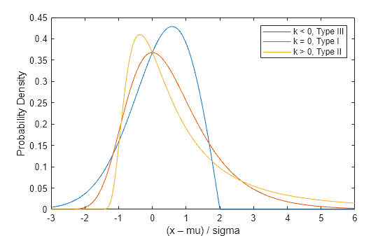
Notice that for k < 0 or k > 0, the density has zero probability above or below, respectively, the upper or lower bound (–1/k). In the limiting case as k approaches 0, the GEV is unbounded. This can be summarized as the constraint that 1 + k*(y – mu)/sigma must be positive.

Simulate Block Maximum Data

The GEV distribution can be defined constructively as the limiting distribution of block maxima (or minima). That is, if you generate a large number of independent random values from a single probability distribution, and take their maximum value, the distribution of that maximum is approximately a GEV.

The original distribution determines the shape parameter, k, of the resulting GEV distribution. Distributions whose tails fall off as a polynomial, such as Student's t, lead to a positive shape parameter. Distributions whose tails decrease exponentially, such as the normal, correspond to a zero shape parameter. Distributions with finite tails, such as the beta, correspond to a negative shape parameter.

Real applications for the GEV distribution might include modeling the largest return for a stock during each month. For this example, simulate data by taking the maximum of 25 values from a Student's t distribution with two degrees of freedom. The simulated data includes 75 random block maximum values.

rng(0,"twister");
y = max(trnd(2,25,75),[],1);

Fit the Distribution Using Maximum Likelihood

The gevfit function returns both maximum likelihood parameter estimates, and (by default) 95% confidence intervals.

[paramEsts,paramCIs] = gevfit(y);

kMLE = paramEsts(1)        % Shape parameter

kMLE = 
0.4901

sigmaMLE = paramEsts(2)    % Scale parameter

sigmaMLE = 
1.4856

muMLE = paramEsts(3)       % Location parameter

muMLE = 
2.9710

kCI = paramCIs(:,1)        % Confidence interval

kCI = 2×1

    0.2020
    0.7782

sigmaCI = paramCIs(:,2)    % Confidence interval

sigmaCI = 2×1

    1.1431
    1.9307

muCI = paramCIs(:,3)       % Confidence interval

muCI = 2×1

    2.5599
    3.3821

Notice that the 95% confidence interval for k does not include the value 0. The type I extreme value distribution is not a good model for these data. That is because the underlying distribution of the simulated data has much heavier tails than a normal distribution, and the type II extreme value distribution is theoretically the correct one as the block size becomes large.

As an alternative to confidence intervals, you can compute an approximation to the asymptotic covariance matrix of the parameter estimates, and from that extract the parameter standard errors.

[nll,acov] = gevlike(paramEsts,y);
paramSEs = sqrt(diag(acov))

paramSEs = 3×1

    0.1470
    0.1986
    0.2097

Examine the Fit

To visually assess the fit, examine the plots of the fitted probability density function (pdf) and cumulative distribution function (cdf).

The support of the GEV depends on the parameter values. In this case, the estimate for k is positive, so the fitted distribution has zero probability below a lower bound.

lowerBnd = muMLE-sigmaMLE./kMLE;

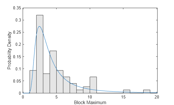
Plot a scaled histogram of the data and add the pdf for the fitted GEV model. To make the histogram comparable to the pdf, scale the histogram so that the bar heights multiplied by their width sum to 1.

ymax = 1.1*max(y);
bins = floor(lowerBnd):ceil(ymax);
h = bar(bins,histc(y,bins)/length(y),"histc");
h.FaceColor = [.9 .9 .9];
ygrid = linspace(lowerBnd,ymax,100);
line(ygrid,gevpdf(ygrid,kMLE,sigmaMLE,muMLE));
xlabel("Block Maximum");
ylabel("Probability Density");
xlim([lowerBnd ymax]);

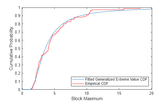
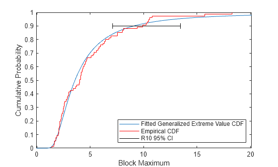
Compare the fit to the data in terms of cumulative probability, by plotting both the empirical cdf and the fitted cdf.

[F,yi] = ecdf(y);
plot(ygrid,gevcdf(ygrid,kMLE,sigmaMLE,muMLE),"-");
hold on;
stairs(yi,F,"r");
hold off;
xlabel("Block Maximum");
ylabel("Cumulative Probability");
legend("Fitted Generalized Extreme Value CDF","Empirical CDF",Location="southeast");
xlim([lowerBnd ymax]);

Estimate Quantiles of the Model

While the parameter estimates may be important by themselves, a quantile of the fitted GEV model is often the quantity of interest in analyzing block maxima data.

For example, the return level Rm is defined as the block maximum value expected to be exceeded only once in m blocks. That is just the (1-1/m)'th quantile. We can plug the maximum likelihood parameter estimates into the inverse CDF to estimate Rm for m=10.

R10MLE = gevinv(1-1./10,kMLE,sigmaMLE,muMLE)

R10MLE = 
9.0724

You can compute confidence limits for R10 using asymptotic approximations, but those may not be valid. Instead, use a likelihood-based method to compute confidence limits. This method often produces more accurate results than one based on the estimated covariance matrix of the parameter estimates.

Given any set of values for the parameters mu, sigma, and k, you can compute a log-likelihood—for example, the MLEs are the parameter values that maximize the GEV log-likelihood. As the parameter values move away from the MLEs, their log-likelihood typically becomes significantly less than the maximum. The set of parameter values that produce a log-likelihood larger than a specified critical value lie in a complicated region of the parameter space. However, for a suitable critical value, it is a confidence region for the model parameters. The region contains parameter values that are "compatible with the data". Because the critical value that determines the region is based on a chi-square approximation, use 95% as the confidence level, and use the negative of the log-likelihood.

nllCritVal = gevlike([kMLE,sigmaMLE,muMLE],y) + .5*chi2inv(.95,1)

nllCritVal = 
170.3044

For any set of parameter values mu, sigma, and k, you can compute R10. Therefore, you can find the smallest R10 value achieved within the critical region of the parameter space where the negative log-likelihood is larger than the critical value. That smallest value is the lower likelihood-based confidence limit for R10.

Because it is difficult to visualize in all three parameter dimensions, you can fix the shape parameter k and see how the procedure would work over the two remaining parameters, sigma and mu.

sigmaGrid = linspace(.8, 2.25, 110);
muGrid = linspace(2.4, 3.6);
nllGrid = zeros(length(sigmaGrid),length(muGrid));
R10Grid = zeros(length(sigmaGrid),length(muGrid));
for i = 1:size(nllGrid,1)
    for j = 1:size(nllGrid,2)
        nllGrid(i,j) = gevlike([kMLE,sigmaGrid(i),muGrid(j)],y);
        R10Grid(i,j) = gevinv(1-1./10,kMLE,sigmaGrid(i),muGrid(j));
    end
end
nllGrid(nllGrid>gevlike([kMLE,sigmaMLE,muMLE],y)+6) = NaN;
contour(muGrid,sigmaGrid,R10Grid,6.14:.64:12.14,LineColor="r");
hold on
contour(muGrid,sigmaGrid,R10Grid,[7.42 11.26],LineWidth=2,LineColor="r");
contour(muGrid,sigmaGrid,nllGrid,[168.7 169.1 169.6 170.3:1:173.3],LineColor="b");
contour(muGrid,sigmaGrid,nllGrid,[nllCritVal nllCritVal],LineWidth=2,LineColor="b");
hold off
axis([2.4 3.6 .8 2.25]);
xlabel("mu");
ylabel("sigma");

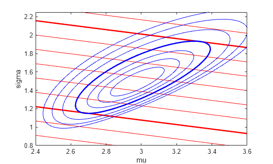
The blue contours represent the log-likelihood surface, and the thick blue contour is the boundary of the critical region. The red contours represent the surface for R10—larger values are to the top right, and lower values are to the bottom left. The red contours are straight lines because Rm is a linear function of sigma and mu when the value of k is fixed. The thick red contours are the lowest and highest values of R10 that fall within the critical region. In the full three dimensional parameter space, the log-likelihood contours are ellipsoidal, and the R10 contours are surfaces.

Finding the lower confidence limit for R10 is an optimization problem with nonlinear inequality constraints. You can use the fmincon function from Optimization Toolbox™. Because you want to find the smallest R10 value, the objective to be minimized is R10 itself, equal to the inverse CDF evaluated for p=1 – 1/m. We'll create a wrapper function that computes Rm specifically for m=10.

CIobjfun = @(params) gevinv(1-1./10,params(1),params(2),params(3));

To perform the constrained optimization, you also need a function that defines the constraint, that is, that the negative log-likelihood be less than the critical value. The constraint function should return positive values when the constraint is violated. Create an anonymous function, using the simulated data and the critical log-likelihood value. The function also returns an empty value because you not using any equality constraints in this optimization problem.

CIconfun = @(params) deal(gevlike(params,y) - nllCritVal, []);

Perform the constrained optimization by calling fmincon using the active-set algorithm.

opts = optimset(Algorithm="active-set",Display="notify",MaxFunEvals=500, ...
    RelLineSrchBnd=0.1,RelLineSrchBndDuration=Inf);
[params,R10Lower,flag,output] = ...
    fmincon(CIobjfun,paramEsts,[],[],[],[],[],[],CIconfun,opts);

Feasible point with lower objective function value found, but optimality criteria not satisfied. See output.bestfeasible..

To find the upper likelihood confidence limit for R10, reverse the sign on the objective function to find the largest R10 value in the critical region, and call fmincon a second time.

CIobjfun = @(params) -gevinv(1-1./10,params(1),params(2),params(3));
[params,R10Upper,flag,output] = ...
    fmincon(CIobjfun,paramEsts,[],[],[],[],[],[],CIconfun,opts);
R10Upper = -R10Upper;

R10CI = [R10Lower, R10Upper]

R10CI = 1×2

    7.0841   13.4452

plot(ygrid,gevcdf(ygrid,kMLE,sigmaMLE,muMLE),"-");
hold on;
stairs(yi,F,"r");
plot(R10CI([1 1 1 1 2 2 2 2]), [.88 .92 NaN .9 .9 NaN .88 .92],"k-")
hold off;
xlabel("Block Maximum");
ylabel("Cumulative Probability");
legend("Fitted Generalized Extreme Value CDF","Empirical CDF", ...
    "R10 95% CI",Location="southeast");
xlim([lowerBnd ymax]);

Likelihood Profile for a Quantile

Sometimes just an interval does not give enough information about the quantity being estimated, and a profile likelihood is needed instead. To find the log-likelihood profile for R10, fix a possible value for R10, and then maximize the GEV log-likelihood with the parameters constrained so that they are consistent with that current value of R10. This is a nonlinear equality constraint. Obtain a likelihood profile by repeating the procedure over a range of R10 values.

As with the likelihood-based confidence interval, you can think about what this procedure would be if you fixed k and worked over the two remaining parameters, sigma and mu. Each red contour line in the contour plot shown earlier represents a fixed value of R10; the profile likelihood optimization consists of stepping along a single R10 contour line to find the highest log-likelihood (blue) contour.

Compute a profile likelihood for R10 over the values that were included in the likelihood confidence interval.

R10grid = linspace(R10CI(1)-.05*diff(R10CI), R10CI(2)+.05*diff(R10CI), 51);

The objective function for the profile likelihood optimization is simply the log-likelihood, using the simulated data.

PLobjfun = @(params) gevlike(params,y);

To use fmincon, you need a function that returns non-zero values when the constraint is violated, that is, when the parameters are not consistent with the current value of R10. For each value of R10, create an anonymous function for the particular value of R10 under consideration. As before, the function also returns an empty value because you not using any equality constraints in this optimization problem.

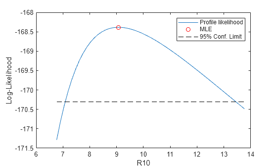
Finally, call fmincon at each value of R10, to find the corresponding constrained maximum of the log-likelihood. Start near the maximum likelihood estimate of R10, and work outwards in both directions.

Lprof = nan(size(R10grid));
params = paramEsts;
[dum,peak] = min(abs(R10grid-R10MLE));
for i = peak:1:length(R10grid)
    PLconfun = ...
        @(params) deal([], gevinv(1-1./10,params(1),params(2),params(3)) - R10grid(i));
    [params,Lprof(i),flag,output] = ...
        fmincon(PLobjfun,params,[],[],[],[],[],[],PLconfun,opts);
end

params = paramEsts;
for i = peak-1:-1:1
    PLconfun = ...
        @(params) deal([], gevinv(1-1./10,params(1),params(2),params(3)) - R10grid(i));
    [params,Lprof(i),flag,output] = ...
        fmincon(PLobjfun,params,[],[],[],[],[],[],PLconfun,opts);
end

plot(R10grid,-Lprof,"-", R10MLE,-gevlike(paramEsts,y),"ro", ...
    [R10grid(1), R10grid(end)],[-nllCritVal,-nllCritVal],"k--");
xlabel("R10");
ylabel("Log-Likelihood");
legend("Profile likelihood","MLE","95% Conf. Limit");