Main Content

nlparci

Nonlinear regression parameter confidence intervals

    Description

    ci = nlparci(beta,r,"Covar",CovB) returns the 95% confidence intervals ci for the nonlinear least-squares parameter estimates beta. Before calling nlparci, get the estimated coefficients beta, residuals r, and estimated covariance matrix CovB by using the nlinfit function to fit a nonlinear regression model.

    If you use a robust option with nlinfit, you must use this syntax for nlparci. The covariance matrix CovB is required with robust fitting.

    ci = nlparci(beta,r,"Jacobian",J) returns the 95% confidence intervals ci for the nonlinear least-squares parameter estimates beta. Before calling nlparci, get the estimated coefficients beta, residuals r, and Jacobian J by using the nlinfit function to fit a nonlinear regression model.

    ci = nlparci(___,"Alpha",alpha) returns the 100(1 — alpha)% confidence intervals, using any of the input argument combinations in the previous syntaxes.

    example

    Examples

    collapse all

    Fit an exponential decay model of the form

    yi=β1+β2exp(-β3xi)+ϵi,

    where βj are the parameters to estimate, xi are the data points, yi are the responses, and εi is the noise term.

    Write a function handle that represents the model.

    mdl = @(beta,x)(beta(1) + beta(2)*exp(-beta(3)*x));

    Generate synthetic data with true parameter values beta = [1;3;2], x data points distributed exponentially with parameter 2, and noise distributed normally with mean 0 and standard deviation 0.1.

    rng(9845,'twister') % For reproducibility
    beta = [1;3;2];
    x = exprnd(2,100,1);
    epsn = normrnd(0,0.1,100,1);
    y = mdl(beta,x) + epsn;

    Fit the model to data starting from the arbitrary value beta0 = [2;2;2].

    beta0 = [2;2;2];
    [betahat,r,J,CovB,mse] = nlinfit(x,y,mdl,beta0);
    betahat
    betahat = 3×1
    
        1.0153
        3.0229
        2.1070


    Check the 95% confidence intervals using the covariance matrix. Note that the true parameter values [1;3;2] are within all three intervals.

    ci = nlparci(betahat,r,"Covar",CovB)
    ci = 3×2
    
        0.9869    1.0438
        2.9401    3.1058
        1.9963    2.2177


    You can obtain the same result using the Jacobian.

    ci = nlparci(betahat,r,"Jacobian",J)
    ci = 3×2
    
        0.9869    1.0438
        2.9401    3.1058
        1.9963    2.2177


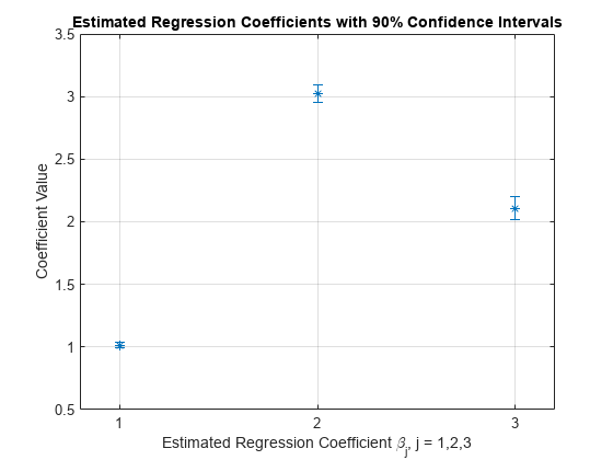
    Determine if the true parameter values [1;3;2] are in the narrower 90% confidence intervals. Note that β1 and β2 are within these intervals, but β3 is not.

    ci = nlparci(betahat,r,"Covar",CovB,"Alpha",0.1)
    ci = 3×2
    
        0.9915    1.0392
        2.9536    3.0923
        2.0144    2.1996


    Plot the estimated regression coefficients with the 90% confidence intervals.

    lowerBars = betahat - ci(:,1);
    upperBars = ci(:,2) - betahat;
    errorbar(1:3,betahat,lowerBars,upperBars,'*'), grid
    title('Estimated Regression Coefficients with 90% Confidence Intervals')
    ylabel('Coefficient Value')
    xlabel('Estimated Regression Coefficient \beta_j, j = 1,2,3')
    xticks([1 2 3])
    xlim([.8 3.2])

    Figure contains an axes object. The axes object with title Estimated Regression Coefficients with 90% Confidence Intervals, xlabel Estimated Regression Coefficient beta indexOf j baseline , blank j blank = 1,2,3, ylabel Coefficient Value contains an object of type errorbar.

    Input Arguments

    collapse all

    Estimated regression coefficients, specified as a numeric vector returned by the nlinfit function.

    Data Types: single | double

    Residuals, specified as a numeric vector returned by the nlinfit function.

    Data Types: single | double

    Estimated covariance matrix for the fitted coefficients beta, specified as a numeric matrix returned by the nlinfit function.

    Data Types: single | double

    Estimated Jacobian, specified as a numeric matrix returned by the nlinfit function.

    Data Types: single | double

    Significance level for the confidence intervals, specified as a scalar value in the range (0,1). The confidence level is 100(1 — alpha)%, where alpha is the probability that the confidence intervals do not contain the true value.

    The default confidence level is 95% (alpha = 0.05).

    Example: "Alpha",0.1

    Data Types: single | double

    Output Arguments

    collapse all

    Confidence intervals for the estimated regression coefficients, returned as an N-by-2 numeric matrix, where N is the number of rows in beta. The first column of ci represents the lower confidence interval bounds, and the second column represents the upper bounds.

    Data Types: single | double

    Algorithms

    • nlparci treats NaN values in the residuals r, or the Jacobian J as missing values, and ignores the corresponding observations.

    • The confidence interval calculation is valid for systems where the length of the residuals r exceeds the length of the coefficients beta, and the Jacobian J has full column rank. When J is ill-conditioned, the confidence intervals might be inaccurate.

    Alternative Functionality

    You can also get the confidence intervals by using the fitnlm function instead of nlinfit and the coefCI function instead of nlparci.

    Version History

    Introduced before R2006a
    See Also

    |

    Go to top of page