Predict Responses Using RegressionGP Predict Block

This example uses:

This example shows how to use the RegressionGP Predict block for response prediction in Simulink®. The block accepts an observation (predictor data) and returns the predicted response for the observation using the trained Gaussian process (GP) regression model. The block can also return the standard deviation and prediction intervals of the response.

Train Regression Model

Train a GP regression model at the MATLAB® command line, and calculate the predicted responses and prediction intervals.

Load the gprdata data set. The data set contains simulated training and test data, with 500 observations in training data and 100 observations in test data. The data has 6 predictor variables.

load gprdata

Train a GP regression model by passing the training data Xtrain and ytrain to the fitrgp function. Specify to standardize the numeric predictors.

gpMdl = fitrgp(Xtrain,ytrain,Standardize=1)

gpMdl = 
  RegressionGP
             ResponseName: 'Y'
    CategoricalPredictors: []
        ResponseTransform: 'none'
          NumObservations: 500
           KernelFunction: 'SquaredExponential'
        KernelInformation: [1x1 struct]
            BasisFunction: 'Constant'
                     Beta: 304.8486
                    Sigma: 0.8235
        PredictorLocation: [6x1 double]
           PredictorScale: [6x1 double]
                    Alpha: [500x1 double]
         ActiveSetVectors: [500x6 double]
            PredictMethod: 'Exact'
            ActiveSetSize: 500
                FitMethod: 'Exact'
          ActiveSetMethod: 'Random'
        IsActiveSetVector: [500x1 logical]
            LogLikelihood: -770.2440
         ActiveSetHistory: []
           BCDInformation: []

gpMdl is a RegressionGP model. You can use dot notation to access the properties of gpMdl. For example, you can specify gpMdl.TrainingHistory to display more information about the training history of the GP model.

Compute the predictions ypred and prediction intervals yint, and calculate the root mean squared error (RMSE).

[ypred,~,yint] = predict(gpMdl,Xtest);
rmse = sqrt(mean((ypred-ytest).^2))

rmse = 
0.9166

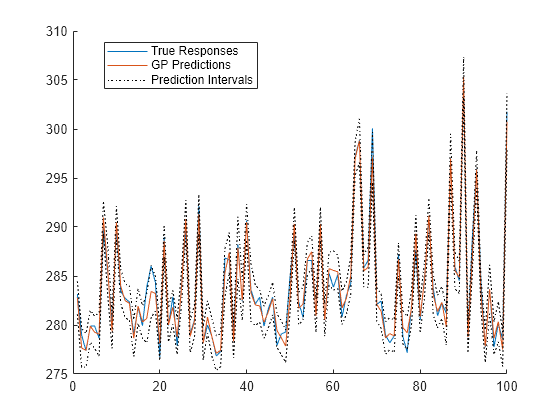
Plot the true responses, predicted responses, and prediction intervals.

hold on
plot(ytest)
plot(ypred)
plot(yint(:,1),"k:")
plot(yint(:,2),"k:")
hold off
legend("True Responses","GP Predictions",...
    "Prediction Intervals",Location="best")

Figure contains an axes object. The axes object contains 4 objects of type line. These objects represent True Responses, GP Predictions, Prediction Intervals.

Now that you have trained the model gpMdl, you can import it into the RegressionGP Predict block.

Create Simulink Model

Create a new model using the RegressionGP Predict block. To create a new Simulink model, open the Blank Model template and add the RegressionGP Predict block from the Statistics and Machine Learning Toolbox™ library.

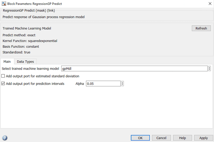
Double-click the RegressionGP Predict block to open the Block Parameters dialog box. Import a trained RegressionGP model into the block by specifying the name of a workspace variable that contains the model. The default variable name is gpMdl, which is the model you trained at the command line.

Click the Refresh button to refresh the settings of the trained model in the dialog box. The Trained Machine Learning Model section of the dialog box displays the options used to train the model gpMdl. Select the check box Add output port for prediction intervals to add a second output port (yint) in the block.

Add one Inport and two Outport blocks, and connect them to the input and outputs of the RegressionGP Predict block.

The RegressionGP Predict block expects an observation containing 6 predictor values, because the model was trained using a data set with 6 predictor variables. Double-click the Inport block, and set Port dimensions to 6 on the Signal Attributes tab. If you want the output signals to have the same length as the input signal, set Sample Time to 1.

Create an input signal in the form of a structure array for the Simulink model. The structure array must contain these fields:

time — The points in time at which the observations enter the model. The orientation must correspond to the observations in the predictor data. In this example, time must be a column vector.
signals — A 1-by-1 structure array describing the input data and containing the fields values and dimensions, where values is a matrix of predictor data, and dimensions is the number of predictor variables.

Create an appropriate structure array for future predictions. For more information, see Structure with Time (Simulink).

modelInput.time = (0:length(ytest)-1)';
modelInput.signals(1).values = Xtest;
modelInput.signals(1).dimensions = size(Xtest,2);

Import the signal data from the workspace:

Open the Configuration Parameters dialog box. On the Modeling tab, click Model Settings.
In the Data Import/Export pane, select the Input check box and enter modelInput in the adjacent text box.
In the Solver pane, under Simulation time, set Stop time to modelInput.time(end). Under Solver selection, set Type to Fixed-step, and set Solver to discrete (no continuous states).

For more details, see Load Signal Data for Simulation (Simulink).

Double-click the Outport 1 block and set Signal name to ypred on the Main tab. Similarly, double-click the Outport 2 block and set Signal name to yint.

Open Provided Model

Instead of creating a new model, you can open the provided Simulink model slexRegressionGPPredictExample.slx, which includes the RegressionGP Predict block. To access this model, you must open the example as a live script.

Open the Simulink model slexRegressionGPPredictExample.slx.

SimMdlName = "slexRegressionGPPredictExample"; 
open_system(SimMdlName)

If you open the Simulink model, then the software runs the code in the PreLoadFcn callback function before loading the Simulink model. The PreLoadFcn callback function of slexRegressionGPPredictExample includes code to check if your workspace contains the gpMdl variable for the trained model. If the workspace does not contain the variable, PreLoadFcn loads the sample data, trains the GP model, and creates an input signal for the Simulink model. To view the callback function, in the Setup section on the Modeling tab, click Model Settings and select Model Properties. Then, on the Callbacks tab, select the PreLoadFcn callback function in the Model callbacks pane.

Simulate Simulink Model

Simulate the Simulink model, and export the simulation outputs to the workspace. When the Inport block detects an observation, it places the observation into the RegressionGP Predict block. You can use the Simulation Data Inspector (Simulink) to view the logged data of the Outport block.

simOut = sim(SimMdlName)

simOut = 
  Simulink.SimulationOutput:
                   tout: [100x1 double] 
                   yout: [1x1 Simulink.SimulationData.Dataset] 

     SimulationMetadata: [1x1 Simulink.SimulationMetadata] 
           ErrorMessage: [0x0 char]

Determine the simulated predictions and prediction intervals, and calculate the RMSE for the simulated predictions.

outputs = simOut.yout;
sim_ypred = outputs.get("ypred").Values.Data;
sim_yint = outputs.get("yint").Values.Data;
sim_rmse = sqrt(mean((sim_ypred-ytest).^2))

sim_rmse = 
0.9166

Plot the true responses, simulated predictions, and simulated prediction intervals.

hold on
plot(ytest,"b")
plot(sim_ypred,"r")
plot(sim_yint(:,1),"k:")
plot(sim_yint(:,2),"k:")
hold off
legend("True Responses","Simulated GP Predictions",...
    "Simulated Prediction Intervals",Location="best")

Figure contains an axes object. The axes object contains 8 objects of type line. These objects represent True Responses, Simulated GP Predictions, Simulated Prediction Intervals.

The plot is similar to the plot created with the outputs of the predict function.

Predict Responses Using RegressionGP Predict Block

Train Regression Model

Create Simulink Model

Open Provided Model

Simulate Simulink Model

See Also

Related Topics