主要内容

responseSurfaceDOE

R2026b

Response surface design of experiments (DOE)

Since R2026b

Description

A responseSurfaceDOE object contains a response surface design for an experiment, as well as information about the design, experiment model, and factors. Create a responseSurfaceDOE object to generate a central composite (Box–Wilson) or Box–Behnken design that is suitable for calibrating a quadratic model of a curved response surface.

Creation

Description

rsdoe = responseSurfaceDOE(n,designType) generates a response surface design of type designType for n factors, and returns the design information in the responseSurfaceDOE object rsdoe. The design type determines the number of levels per factor. Depending on the design type, a response surface design can contain factorial points, edge points, star points, and center points, where each point is a combination of factor level values that corresponds to a run in the design. For more information, see Response Surface Designs.

example

rsdoe = responseSurfaceDOE(Bounds,designType) specifies the number of factors and the bounds for the design points (runs).

example

rsdoe = responseSurfaceDOE(___,Name=Value) specifies options using one or more name-value arguments in addition to any of the input argument combinations in the previous syntaxes. For example, you can specify the experiment model and the number of center points.

example

Input Arguments

expand all

Number of factors in the design, specified as a positive integer. n must be greater than or equal to 2 (or 3, if designType is "box-behnken"). You can also specify the number of factors by setting Bounds.

Data Types: single | double

Type of response surface design, specified as a value in the following table.

ValueLevels Per FactorDescription
"cc-circumscribed"5Circumscribed central composite design consisting of factorial (corner) points, star points, and central points. Each point corresponds to a run in the design.
"cc-faced"3Same as "cc-circumscribed", but with the star point-to-center distances scaled by a factor K=(2^(n – FractionalDesignIndex))^(–0.25), where n is the number of factors in the design
"cc-inscribed"5Same as "cc-circumscribed", but with all of the point-to-center distances scaled by K
"box-behnken"3Box–Behnken design. The points are located at the midpoints of the design space edges and at the center, and do not contain an embedded factorial design.

For more information about design types, see Response Surface Designs.

This argument sets the DesignType property.

Level bounds, specified as a 2-by-n numeric matrix, where n is the number of factors in the design. Each column of Bounds corresponds to a factor. The first row of Bounds contains the lower bounds, and the second row contains the upper bounds. If designType is "cc-circumscribed", the bounds do not apply to the star points.

This argument sets the Bounds property.

Data Types: single | double

Name-Value Arguments

expand all

Specify optional pairs of arguments as Name1=Value1,...,NameN=ValueN, where Name is the argument name and Value is the corresponding value. Name-value arguments must appear after other arguments, but the order of the pairs does not matter.

Example: responseSurfaceDOE(4,"box-behnken",CenterPoints=6) generates a Box–Behnken design for four factors with six center points.

Number of center points, specified as a nonnegative integer, "orthogonal", or "uniform".

  • Nonnegative integer –- The function generates a design with the specified number of center points.

  • "orthogonal" –- The function selects the number of center points needed for an orthogonal design, based on the values of n and FractionalDesignIndex (see [4]). An orthogonal design allows the main effects, interaction effects, and quadratic effects in the model to be estimated independently. You cannot specify "orthogonal" if designType is "box-behnken". For more information about model effects, see Fractional Factorial Designs.

  • "uniform" –- The function selects the number of center points needed for a design with uniform precision, based on the values of n and FractionalDesignIndex (see [4]). In a uniform precision design, the variance of the predicted response does not depend on the distance from the center point. You cannot specify "uniform" if designType is "box-behnken".

When designType is any value other than "box-behnken", the default value of CenterPoints is "orthogonal". Otherwise, the default value of CenterPoints depends on the number of factors.

This argument sets the CenterPoints property.

Example: CenterPoints=2

Data Types: single | double | string array

Factor names, specified as a string vector or a cell array of character vectors. The number of unique values in FactorNames must equal the number of factors in the design. The default value for FactorNames is ["Factor1","Factor2",..."FactorN"].

If you specify ModelSpecification as a character vector or string scalar formula in Wilkinson Notation, then FactorNames must contain only valid variable names.

Example: FactorNames=["compound","quantity"]

Data Types: char | string | cell

Fractional design index, specified as an integer scalar in the range [0,4]. If FractionalDesignIndex > 0, the function generates a central component design that is (0.5)^FractionalDesignIndex of the full factorial cube. You cannot specify FractionalDesignIndex if designType is "box-behnken".

The default value and allowable values of FractionalDesignIndex depend on the number of factors n. For example, if n > 11, you can only specify FractionalDesignIndex as 0 or 1.

Number of FactorsDefault Value of FractionalDesignIndex and Design FractionAllowable Values of FractionalDesignIndex
2 ≤ n ≤ 40 (Entire cube)0
5 ≤ n ≤ 71 (1/2 of cube)0,1
8 ≤ n ≤ 92 (1/4 of cube)0,1,2
n = 103 (1/8 of cube)0,1,2,3
n = 114 (1/16 of cube)0,1,2,3,4
n > 110 (Entire cube)0,1

This argument sets the FractionalDesignIndex property.

Example: FractionalDesignIndex=3

Data Types: single | double

Maximum number of points per block, specified as a positive integer. If you specify a MaxBlockSize value other than Inf (the default), the function attempts to create a blocked design in which no block has more than MaxBlockSize points. The function stores the block index of each point in the BlockIndices property. To specify the number of blocks in the design, use NumBlocks.

If you specify MaxBlockSize and do not specify NumBlocks, the function attempts to create a blocked design that minimizes the number of blocks, while restricting each block to no more than MaxBlockSize points.

Example: MaxBlockSize=8

Data Types: single | double

Experiment model, specified as one of the following values.

  • A character vector or string scalar with the model name.

    ValueModel Description
    "linear"The model contains an intercept and linear term for each factor.
    "interactions"The model contains an intercept, a linear term for each factor, and all products of pairs of distinct factors (no squared terms).
    "purequadratic"The model contains an intercept term, and linear and squared terms for each factor.
    "quadratic" (default)The model contains an intercept term, linear and squared terms for each factor, and all products of pairs of distinct factors.
    "scheffe-linear"

    The model contains a linear term for each factor and does not include an intercept term.

    "scheffe-quad"

    The model is given by the formula:

    i=1nbixi+i=1nj<in1bijxixj

    "scheffe-special-cubic"

    The model is given by the formula:

    i=1nbixi+i=1nj<in1bijxixj+i=1nj<in1k<jn2bijkxixjxk

    "polyijk"The model is a polynomial with all terms up to degree i in the first factor, degree j in the second factor, and so on. Specify the maximum degree for each factor by using numerals 0 though 9. The model contains interaction terms, but the degree of each interaction term does not exceed the maximum value of the specified degrees. For example, "poly13" has an intercept and x1, x2, x22, x23, x1*x2, and x1*x22 terms, where x1 and x2 are the first and second factors, respectively.

    In the above table, each xi corresponds to the ith factor in the design, and bi, bij, and bijk are coefficients for the model terms.

  • A character vector or string scalar formula in Wilkinson notation. The factor names in the formula must be valid variable names specified by FactorNames.

  • A t-by-n terms matrix, where t is the number of terms and n is the number of factors in the design. A terms matrix is convenient when the number of factors is large and you want to generate the terms programmatically. For more information, see Terms Matrix.

ModelSpecification does not include the response variable.

This argument sets the ModelSpecification property.

Example: ModelSpecification="interactions"

Example: ModelSpecification="Factor1 + Factor2 + Factor1:Factor2"

Data Types: single | double | char | string

Number of blocks in the blocked design, specified as a nonnegative integer. The blocks indicate the points (runs) to measure under similar conditions in order to minimize the effect of inter-block differences on the parameter estimates. The allowable values for NumBlocks depend on the design type and other parameter settings. The function stores the block index of each point in the BlockIndices property. If you do not specify MaxBlockSize or specify MaxBlockSize=Inf, the default value of NumBlocks is 0. Otherwise, the default value of NumBlocks depends on the value of MaxBlockSize.

Example: NumBlocks=2

Data Types: single | double

Output Arguments

expand all

Response surface design, returned as a responseSurfaceDOE object.

Properties

expand all

This property is read-only after object creation.

Block indices for each point (run), specified as an m-by-1 numeric vector, where m is the number of runs in the design. The blocks indicate the runs to measure under similar conditions in order to minimize the effect of inter-block differences on the parameter estimates. You can set block indices using the NumBlocks or MaxBlockSize name-value arguments. For more information about blocked designs, see [2].

This property is read-only after object creation.

Values of the input bounds, specified as a 2-by-n numeric array, where n is the number of factors in the design. If you do not specify the Bounds argument when you create rsdoe, then each column of Bounds is [-1; 1].

This property is read-only after object creation.

Number of center points in the design, specified as a nonnegative integer, "orthogonal", or "uniform".

This property is read-only after object creation.

Generated design runs (points), specified as a table. Each column of Design corresponds to a factor in the design, and each row corresponds to a run. You can randomize the order of the design runs using the randomizeRunOrder function, and add replicates to the design using the addReplicates function.

This property is read-only after object creation.

Design type, specified as "cc-circumscribed", "cc-inscribed", "cc-faced", or "box-behnken".

This property is read-only after object creation.

Fractional design index, specified as an integer scalar in the range [0,4].

Since R2026b

This property is read-only after object creation. To change the property value, use the randomizeRunOrder function.

Flag indicating whether the run order is randomized, specified as logical 0 (false) or 1 (true). The nonrandomized run order is stored in the StandardRunOrder property.

This property is read-only after object creation.

Experiment model, specified as a formula in Wilkinson notation. ModelSpecification indicates the model you want to fit with the specified design. ModelSpecification does not include the response variable.

Since R2026b

This property is read-only after object creation. To change the property value, use the addReplicates function.

Number of replicates, specified as a nonnegative integer. A replicate is a duplicate of the original runs in the responseSurfaceDOE object when it is created.

Since R2026b

This property is read-only after object creation. To change the property value, use the randomizeRunOrder function.

Nonrandomized run order, specified as an r-by-1 array of positive integers, where r is the number of runs in the design. You can display the design of the output object rsdoe in nonrandomized run order using rsdoe.Design(rsdoe.StandardRunOrder',:).

Object Functions

addReplicatesAdd replicates to design of experiments (DOE) object
fitlmFit linear regression model using design runs
randomizeRunOrderRandomize run order of design of experiments (DOE) object

Examples

collapse all

Create a faced central composite design for three factors.

rsdoe = responseSurfaceDOE(3,"cc-faced")
rsdoe = 
  responseSurfaceDOE with properties:

                   Design: [24×3 table]
         StandardRunOrder: [24×1 double]
       ModelSpecification: "1 + Factor1*Factor2 + Factor1*Factor3 + Factor2*Factor3 + Factor1^2 + Factor2^2 + Factor3^2"
               DesignType: "cc-faced"
             BlockIndices: []
                   Bounds: [2×3 double]
             CenterPoints: "orthogonal"
    FractionalDesignIndex: 0
             IsRandomized: 0
            NumReplicates: 0

rsdoe is a responseSurfaceDOE object that contains information about the generated design. The output displays the size of the table containing the design and factors. The output also displays the default model specification, which does not affect how the software generates design runs.

Visualize the design using the plot3 function.

plot3(rsdoe.Design.Factor1,rsdoe.Design.Factor2, ...
rsdoe.Design.Factor3,"ro",MarkerFaceColor="b")
line([0 0],[0,0],[-1 1],Color="r")
line([-1 1],[0,0],[0 0],Color="r")
line([0 0],[-1,1],[0 0],Color="r")
xlabel("Factor1")
ylabel("Factor2")
zlabel("Factor3")
set(gca,Box="on",BoxStyle="full")
axis square equal
view([-40,20])
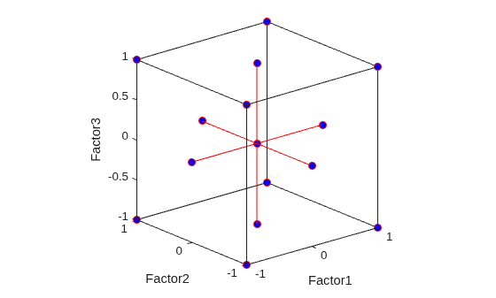
Figure contains an axes object. The axes object with xlabel Factor1, ylabel Factor2 contains 4 objects of type line. One or more of the lines displays its values using only markers

In a faced central composite design, each factor has three levels. Each blue marker (point) in the plot corresponds to the factor settings for a run in the design. The factorial points are located at the vertices of the cube. The star points are located at the center of each cube face, and are connected to the center points with red lines.

By default, the function creates an orthogonal design, which requires multiple center points. Display the number of center points in the design.

nCenter = sum(all(table2array(rsdoe.Design)==0,2))
nCenter = 
10

Create a Box–Behnken design for three factors with levels between 0 and 2.

rsmdoe = responseSurfaceDOE([0 0 0; 2 2 2],"box-behnken")
rsmdoe = 
  responseSurfaceDOE with properties:

                Design: [15×3 table]
      StandardRunOrder: [15×1 double]
    ModelSpecification: "1 + Factor1*Factor2 + Factor1*Factor3 + Factor2*Factor3 + Factor1^2 + Factor2^2 + Factor3^2"
            DesignType: "box-behnken"
          BlockIndices: []
                Bounds: [2×3 double]
          CenterPoints: 3
          IsRandomized: 0
         NumReplicates: 0

rsmdoe is a responseSurfaceDOE object that contains information about the generated design. The output displays the size of the table containing the design and factors. The output also displays the default model specification, which does not affect how the software generates design runs.

Visualize the design using the plot3 function.

plot3(rsmdoe.Design.Factor1,rsmdoe.Design.Factor2, ...
rsmdoe.Design.Factor3,"ro",MarkerFaceColor="b")
xlim([0 1]);
ylim([0 1]);
zlim([0 1]);
xlabel("Factor1")
ylabel("Factor2")
zlabel("Factor3")
set(gca,Box="on",BoxStyle="full")
axis square equal
view([-40,20])
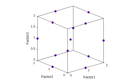
Figure contains an axes object. The axes object with xlabel Factor1, ylabel Factor2 contains a line object which displays its values using only markers.

In a Box–Behnken design, each factor has three levels. Each blue marker (point) in the plot corresponds to the factor settings for a run in the design. With the exception of the center points at (1,1,1), the design points are located at the midpoints of the cube edges.

By default, the function creates an orthogonal design, which requires multiple center points. Display the number of center points in the design.

nCenter = sum(all(table2array(rsmdoe.Design)==1,2))
nCenter = 
3

Create a circumscribed central composite design for two factors with two blocks.

rsmdoe = responseSurfaceDOE(2,"cc-circumscribed",NumBlocks=2)
rsmdoe = 
  responseSurfaceDOE with properties:

                   Design: [16×2 table]
         StandardRunOrder: [16×1 double]
       ModelSpecification: "1 + Factor1*Factor2 + Factor1^2 + Factor2^2"
               DesignType: "cc-circumscribed"
             BlockIndices: [16×1 double]
                   Bounds: [2×2 double]
             CenterPoints: "orthogonal"
    FractionalDesignIndex: 0
             IsRandomized: 0
            NumReplicates: 0

rsmdoe is a responseSurfaceDOE object that contains information about the generated design. The output displays the size of the table containing the design and factors. The output also displays the default model specification, which does not affect how the software generates design runs.

Display the runs in each block.

block1 = rsmdoe.Design(rsmdoe.BlockIndices==1,:)
block1 = 8×2 table
    Factor1    Factor2
    _______    _______

      -1         -1   
      -1          1   
       1         -1   
       1          1   
       0          0   
       0          0   
       0          0   
       0          0   

block2 = rsmdoe.Design(rsmdoe.BlockIndices==2,:)
block2 = 8×2 table
    Factor1    Factor2
    _______    _______

    -1.4142          0
     1.4142          0
          0    -1.4142
          0     1.4142
          0          0
          0          0
          0          0
          0          0

Because the function creates an orthogonal design by default, four of the runs in each block are center points.

Visualize the design using the plot function. Use blue markers for the points in the first block and red markers for the points in the second block. Because both blocks contain center points, use a black marker for the center points.

plot(block1.Factor1,block1.Factor2,"o",MarkerFaceColor="b")
hold on
plot(block2.Factor1,block2.Factor2,"o",MarkerFaceColor="r")
plot(0,0,"ko",MarkerFaceColor="k")
X = [1 -1 -1 -1; 1 1 1 -1];
Y = [-1 -1 1 -1; 1 -1 1 1];
line(X,Y,Color="b")
xlabel("Factor1")
ylabel("Factor2")
axis square equal
hold off
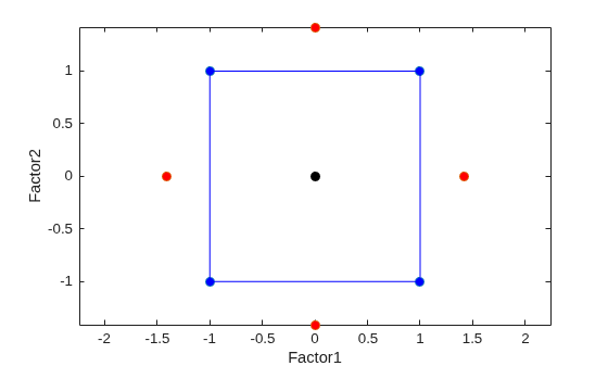
Figure contains an axes object. The axes object with xlabel Factor1, ylabel Factor2 contains 7 objects of type line. One or more of the lines displays its values using only markers

The coordinates of each point represent the factor settings of a run in the design. In the circumscribed design, the points in block 1 form a square, and the points in block 2 are located outside the square.

More About

expand all

References

[1] Box, G. E. P., and K. B. Wilson. "On the Experimental Attainment of Optimum Conditions." Journal of the Royal Statistical Society: Series B (Methodological) 13, no. 1 (January 1951): 1–38. https://doi.org/10.1111/j.2517-6161.1951.tb00067.x.

[2] Box, G. E. P., W. G. Hunter, and J. S. Hunter. Statistics for Experimenters. Hoboken, NJ: Wiley-Interscience, 1978.

[3] Box, G. E. P., and D. Behnken. "Some New Three Level Designs for the Study of Quantitative Variables." Technometrics 2, no. 4 (November 1960): 455–75.

[4] Box, G. E. P., W. G. Hunter, and J. S. Hunter. "Multi-Factor Experimental Designs for Exploring Response Surfaces." Annals of Mathematical Statistics 28, no. 1 (March 1957): 195–241. https://doi.org/10.1214/aoms/1177707047.

Version History

Introduced in R2026b