plot
Plot receiver operating characteristic (ROC) curves and other performance curves
Since R2022a
Syntax
Description
plot( creates
a receiver operating characteristic (ROC) curve, which is a plot of the true positive
rate (TPR) versus the false positive rate (FPR), for each class in the rocObj)ClassNames property of the
rocmetrics object
rocObj. The function marks the model operating point for each
curve, and displays the value of the area under the ROC curve (AUC) and the class name for the curve in the legend.
plot(___, specifies
additional options using one or more name-value arguments in addition to any of the input
argument combinations in the previous syntaxes. For example,
Name=Value)AverageCurveType="macro",ClassNames=[] computes the average
performance metrics using the macro-averaging method and plots the average ROC curve
only.
[ also returns graphics objects for the model operating points and diagonal line.curveObj,graphicsObjs] = plot(___)
Examples
Create a rocmetrics object for a multiclass classification problem, and plot a ROC curve for each class.
Load the fisheriris data set. The matrix meas contains flower measurements for 150 different flowers. The vector species lists the species for each flower. species contains three distinct flower names.
load fisheririsTrain a classification tree that classifies observations into one of the three labels. Cross-validate the model using 10-fold cross-validation.
rng("default") % For reproducibility
Mdl = fitctree(meas,species,Crossval="on");
Compute the classification scores for validation-fold observations.
[~,Scores] = kfoldPredict(Mdl);
size(Scores)
ans = 1×2

   150     3
Scores is a matrix of size 150-by-3. The column order of Scores follows the class order in Mdl. Display the class order stored in Mdl.ClassNames.
Mdl.ClassNames
ans = 3×1 cell
    {'setosa'    }
    {'versicolor'}
    {'virginica' }
Create a rocmetrics object by using the true labels in species and the classification scores in Scores. Specify the column order of Scores using Mdl.ClassNames.
rocObj = rocmetrics(species,Scores,Mdl.ClassNames);
Plot the ROC curve for each class.
plot(rocObj)
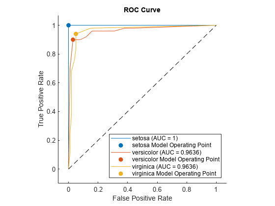
For each class, the plot function plots a ROC curve and displays a filled circle marker at the model operating point. The legend displays the class name and AUC value for each curve.
Plot the average ROC curve by using the plot function. Use a ROCCurve object, an output of the plot function, to obtain the average metric values.
Load the fisheriris data set. The matrix meas contains flower measurements for 150 different flowers. The vector species lists the species for each flower. species contains three distinct flower names.
load fisheririsTrain a classification tree that classifies observations into one of the three labels. Cross-validate the model using 10-fold cross-validation.
rng("default") % For reproducibility
Mdl = fitctree(meas,species,Crossval="on");
Compute the classification scores for validation-fold observations.
[~,Scores] = kfoldPredict(Mdl);
Create a rocmetrics object.
rocObj = rocmetrics(species,Scores,Mdl.ClassNames);
Plot the ROC curve for each class. Specify AverageCurveType="macro" to compute metrics for the average ROC curve using the macro-averaging method.
curveObj = plot(rocObj,AverageCurveType="macro")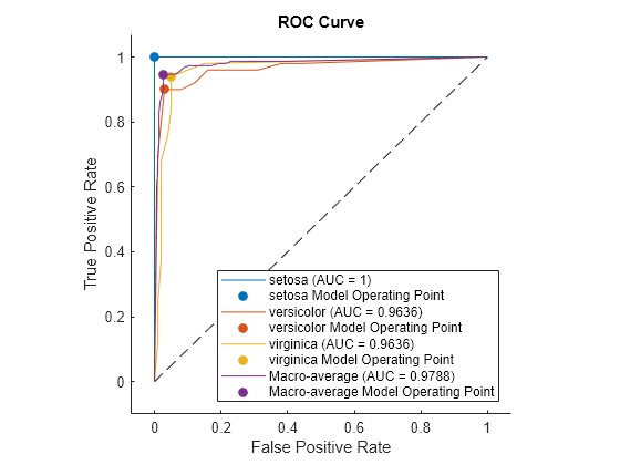
curveObj =
  4×1 ROCCurve array:

  ROCCurve    (setosa (AUC = 1))
  ROCCurve    (versicolor (AUC = 0.9636))
  ROCCurve    (virginica (AUC = 0.9636))
  ROCCurve    (Macro-average (AUC = 0.9788))
The plot function returns a ROCCurve object for each performance curve. You can use the object to query and set properties of the plot after creating it.
Display the data points of the average ROC curve stored in the fourth element of curveObj.
tbl_average = table(curveObj(4).Thresholds,curveObj(4).XData,curveObj(4).YData, ...
    VariableNames=["Threshold",curveObj(4).XAxisMetric,curveObj(4).YAxisMetric])
tbl_average=33×3 table
    Threshold    FalsePositiveRate    TruePositiveRate
    _________    _________________    ________________

           1                 0                  0
           1         0.0066667            0.60667
     0.95455              0.01               0.64
     0.95349              0.01               0.68
     0.95238          0.013333            0.72667
     0.95122          0.013333            0.82667
     0.91304          0.016667               0.86
     0.91111          0.023333            0.88667
     0.86957          0.026667            0.91333
         0.6          0.026667            0.92667
     0.33333          0.026667               0.94
         0.2          0.026667            0.94667
        -0.2              0.03            0.94667
    -0.33333          0.036667            0.94667
        -0.6          0.043333            0.94667
        -0.6          0.046667            0.94667
      ⋮
Create a rocmetrics object and plot performance curves by using the plot function. Specify the XAxisMetric and YAxisMetric name-value arguments of the plot function to plot different types of performance curves other than the ROC curve. If you specify new metrics when you call the plot function, the function computes the new metrics and then uses them to plot the curve.
Load the ionosphere data set. This data set has 34 predictors (X) and 351 binary responses (Y) for radar returns, either bad ('b') or good ('g').
load ionospherePartition the data into training and test sets. Use approximately 80% of the observations to train a support vector machine (SVM) model, and 20% of the observations to test the performance of the trained model on new data. Partition the data using cvpartition.
rng("default") % For reproducibility of the partition
c = cvpartition(Y,Holdout=0.20);
trainingIndices = training(c); % Indices for the training set
testIndices = test(c); % Indices for the test set
XTrain = X(trainingIndices,:);
YTrain = Y(trainingIndices);
XTest = X(testIndices,:);
YTest = Y(testIndices);
Train an SVM classification model.
Mdl = fitcsvm(XTrain,YTrain);
Compute the classification scores for the test set.
[~,Scores] = predict(Mdl,XTest);
Create a rocmetrics object. The rocmetrics function computes the FPR and TPR at different thresholds.
rocObj = rocmetrics(YTest,Scores,Mdl.ClassNames);
Plot the precision-recall curve for the first class. Specify the y-axis metric as precision (or positive predictive value) and the x-axis metric as recall (or true positive rate). The plot function computes the new metric values and plots the curve. Show the model operating point by setting the ShowModelOperatingPoint name-value argument to true.
curveObj = plot(rocObj,ClassNames=Mdl.ClassNames(1), ...
    YAxisMetric="PositivePredictiveValue",XAxisMetric="TruePositiveRate",...
    ShowModelOperatingPoint=true);

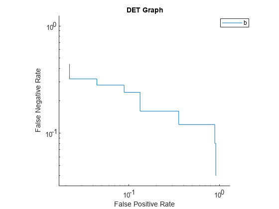
Plot the detection error tradeoff (DET) graph for the first class. Specify the y-axis metric as the false negative rate and the x-axis metric as the false positive rate. Use a log scale for the x-axis and y-axis.
f = figure;
plot(rocObj,ClassNames=Mdl.ClassNames(1), ...
    YAxisMetric="FalseNegativeRate",XAxisMetric="FalsePositiveRate")
f.CurrentAxes.XScale = "log";
f.CurrentAxes.YScale = "log";
title("DET Graph")
Compute the confidence intervals for FPR and TPR for fixed threshold values by using bootstrap samples, and plot the confidence intervals for TPR on the ROC curve.
Load the fisheriris data set. The matrix meas contains flower measurements for 150 different flowers. The vector species lists the species for each flower. species contains three distinct flower names.
load fisheririsTrain a naive Bayes model that classifies observations into one of the three labels. Cross-validate the model using 10-fold cross-validation.
rng("default") % For reproducibility
Mdl = fitcnb(meas,species,Crossval="on");
Compute the classification scores for validation-fold observations.
[~,Scores] = kfoldPredict(Mdl);
Create a rocmetrics object. Specify NumBootstraps as 100 to use 100 bootstrap samples to compute the confidence intervals.
rocObj = rocmetrics(species,Scores,Mdl.ClassNames, ...
    NumBootstraps=100);
Plot the ROC curve and the confidence intervals for TPR. Specify ShowConfidenceIntervals=true to show the confidence intervals.
plot(rocObj,ShowConfidenceIntervals=true)
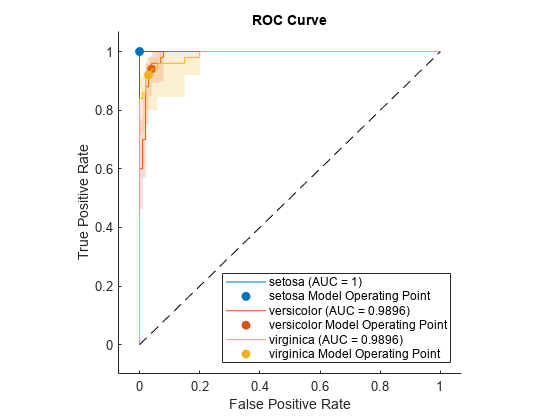
The shaded area around each curve indicates the confidence intervals. The widths of the confidence intervals for setosa are 0 for nonzero false positive rates, so the plot does not have a shaded area for setosa.
rocmetrics computes the ROC curves from the cross-validated scores. Therefore, each ROC curve represents an estimate of a ROC curve on unseen test data for a model trained on the full data set (meas and species). The confidence intervals represent the estimates of uncertainty for the curve. This uncertainty is due to the variance in unseen test data for the model trained on the full data set.
Compute the performance metrics (FPR and TPR) for a binary classification problem by creating a rocmetrics object, and plot a ROC curve by using the plot function. The plot function displays a filled circle at the model operating point. Display a data tip at the model operating point.
Load the ionosphere data set. This data set has 34 predictors (X) and 351 binary responses (Y) for radar returns, either bad ('b') or good ('g').
load ionospherePartition the data into training and test sets. Use approximately 80% of the observations to train a support vector machine (SVM) model, and 20% of the observations to test the performance of the trained model on new data. Partition the data using cvpartition.
rng("default") % For reproducibility of the partition
c = cvpartition(Y,Holdout=0.20);
trainingIndices = training(c); % Indices for the training set
testIndices = test(c); % Indices for the test set
XTrain = X(trainingIndices,:);
YTrain = Y(trainingIndices);
XTest = X(testIndices,:);
YTest = Y(testIndices);
Train an SVM classification model.
Mdl = fitcsvm(XTrain,YTrain);
Compute the classification scores for the test set.
[~,Scores] = predict(Mdl,XTest);
Create a rocmetrics object.
rocObj = rocmetrics(YTest,Scores,Mdl.ClassNames);
The rocmetrics function computes the FPR and TPR at different thresholds and finds the AUC value.
Plot the ROC curve. Specify ClassNames to plot the curve for the first class.
curveObj = plot(rocObj,ClassNames=Mdl.ClassNames(1));
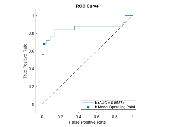
The plot function returns a ROCCurve object for each performance curve. You can use the object to query and set the properties of the plot after creating it.
The filled circle marker indicates the model operating point at which the threshold value is 0. The function chooses a point that has the largest threshold value less than or equal to 0. The legend displays the class name and AUC value for the curve.
You can create data tips by clicking data points on the curve. Alternatively, you can create data tips using the datatip function.
Find the model operating point in the Metrics property of rocObj for class b. The predict function classifies an observation into the class yielding a larger score, which corresponds to the class with a nonnegative adjusted score. That is, the typical threshold value used by the predict function is 0. Among the rows in the Metrics property of rocObj for class b, find the point that has the smallest nonnegative threshold value. The point on the curve indicates identical performance to the performance of the threshold value 0.
idx_b = strcmp(rocObj.Metrics.ClassName,"b");
t = rocObj.Metrics(idx_b,:);
X = rocObj.Metrics(idx_b,:).FalsePositiveRate;
Y = rocObj.Metrics(idx_b,:).TruePositiveRate;
T = rocObj.Metrics(idx_b,:).Threshold;
idx_model = find(T>=0,1,"last");
modelpt = [T(idx_model) X(idx_model) Y(idx_model)]
modelpt = 1×3

    0.1045    0.0222    0.6800
Display a data tip at the model operating point. Specify the target graph object as the output object of the plot function.
datatip(curveObj,DataIndex=idx_model,Location="southeast");
Input Arguments
Object evaluating classification performance, specified as a rocmetrics
object.
Name-Value Arguments
Specify optional pairs of arguments as
Name1=Value1,...,NameN=ValueN, where Name is
the argument name and Value is the corresponding value.
Name-value arguments must appear after other arguments, but the order of the
pairs does not matter.
Example: plot(rocObj,YAxisMetric="PositivePredictiveValue",XAxisMetric="TruePositiveRate")
plots the precision (positive predictive value) versus the recall (true positive rate),
which represents a precision-recall curve.
Since R2024b
Method for averaging ROC or other performance curves, specified as
"none", "micro", "macro",
"weighted", a string array of method names, or a cell array of
method names.
If you specify
"none"(default), theplotfunction does not create the average performance curve.If you specify multiple methods as a string array or a cell array of character vectors, then the
plotfunction plots multiple average performance curves using the specified methods.If you specify one or more averaging methods and specify
ClassNames=[], then theplotfunction plots only the average performance curves.
plot computes the averages of performance metrics for a
multiclass classification problem, and plots the average performance curves using these
methods:
"micro"(micro-averaging) —plotfinds the average performance metrics by treating all one-versus-all binary classification problems as one binary classification problem. The function computes the confusion matrix components for the combined binary classification problem, and then computes the average metrics (as specified by theXAxisMetricandYAxisMetricname-value arguments) using the values of the confusion matrix."macro"(macro-averaging) —plotcomputes the average values for the metrics by averaging the values of all one-versus-all binary classification problems."weighted"(weighted macro-averaging) —plotcomputes the weighted average values for the metrics using the macro-averaging method and using the prior class probabilities (thePriorproperty ofrocObj) as weights.
The algorithm type determines the length of the vectors in the XData, YData, and
Thresholds
properties of a ROCCurve object, returned by plot,
for the average performance curve. For more details, see Average of Performance Metrics.
Example: AverageCurveType="macro"
Example: AverageCurveType=["micro","macro"]
Data Types: char | string | cell
Class labels to plot, specified as a categorical, character, or string array, logical or
numeric vector, or cell array of character vectors. The values and data types in
ClassNames must match those of the class names in the ClassNames property
of rocObj. (The software treats character or string arrays as cell arrays of character vectors.)
If you specify multiple class labels, the
plotfunction plots a ROC curve for each class.If you specify
ClassNames=[]and specify one or more averaging methods usingAverageCurveType, then theplotfunction plots only the average ROC curves.
Example: ClassNames=["red","blue"]
Data Types: single | double | logical | char | string | cell | categorical
Flag to show the confidence intervals of the y-axis metric
(YAxisMetric), specified as a numeric or logical
0 (false) or 1
(true).
The ShowConfidenceIntervals value can be true only if
the Metrics property of
rocObj contains the confidence intervals for the
y-axis metric.
Example: ShowConfidenceIntervals=true
Data Types: single | double | logical
Flag to show the diagonal line that extends from [0,0] to
[1,1], specified as a numeric or logical 1
(true) or 0 (false).
The default value is true if you plot a ROC curve or an average ROC curve, and false otherwise.
In the ROC curve plot, the diagonal line represents a random classifier, and the line passing through [0,0], [0,1], and [1,1] represents a perfect classifier.
Example: ShowDiagonalLine=false
Data Types: single | double | logical
Flag to show the model operating point, specified as a
numeric or logical 1
(true) or 0
(false).
The default value is true for a ROC curve, and false
otherwise.
Example: ShowModelOperatingPoint=false
Data Types: single | double | logical
Metric for the x-axis, specified as a character vector or string scalar of the built-in metric name or a custom metric name, or a function handle (@metricName).
Built-in metrics — Specify one of the following built-in metric names by using a character vector or string scalar.
Name Description "TruePositives"or"tp"Number of true positives (TP) "FalseNegatives"or"fn"Number of false negatives (FN) "FalsePositives"or"fp"Number of false positives (FP) "TrueNegatives"or"tn"Number of true negatives (TN) "SumOfTrueAndFalsePositives"or"tp+fp"Sum of TP and FP "RateOfPositivePredictions"or"rpp"Rate of positive predictions (RPP), (TP+FP)/(TP+FN+FP+TN)"RateOfNegativePredictions"or"rnp"Rate of negative predictions (RNP), (TN+FN)/(TP+FN+FP+TN)"Accuracy"or"accu"Accuracy, (TP+TN)/(TP+FN+FP+TN)"TruePositiveRate","tpr", or"recall"True positive rate (TPR), also known as recall or sensitivity, TP/(TP+FN)"FalseNegativeRate","fnr", or"miss"False negative rate (FNR), or miss rate, FN/(TP+FN)"FalsePositiveRate"or"fpr"False positive rate (FPR), also known as fallout or 1-specificity, FP/(TN+FP)"TrueNegativeRate","tnr", or"spec"True negative rate (TNR), or specificity, TN/(TN+FP)"PositivePredictiveValue","ppv","prec", or"precision"Positive predictive value (PPV), or precision, TP/(TP+FP)"NegativePredictiveValue"or"npv"Negative predictive value (NPV), TN/(TN+FN)"f1score"F1 score, 2*TP/(2*TP+FP+FN)"ExpectedCost"or"ecost"Expected cost,
(TP*cost(P|P)+FN*cost(N|P)+FP*cost(P|N)+TN*cost(N|N))/(TP+FN+FP+TN), wherecostis a 2-by-2 misclassification cost matrix containing[0,cost(N|P);cost(P|N),0].cost(N|P)is the cost of misclassifying a positive class (P) as a negative class (N), andcost(P|N)is the cost of misclassifying a negative class as a positive class.The software converts the
K-by-Kmatrix specified by theCostname-value argument ofrocmetricsto a 2-by-2 matrix for each one-versus-all binary problem. For details, see Misclassification Cost Matrix.The software computes the scale vector using the prior class probabilities (
Prior) and the number of classes inLabels, and then scales the performance metrics according to this scale vector. For details, see Performance Metrics.Custom metric stored in the
Metricsproperty — Specify the name of a custom metric stored in theMetricsproperty of the input objectrocObj. Therocmetricsfunction names a custom metric"CustomMetricN", whereNis the number that refers to the custom metric. For example, specifyXAxisMetric="CustomMetric1"to use the first custom metric inMetricsas a metric for the x-axis.Custom metric — Specify a new custom metric by using a function handle. A custom function that returns a performance metric must have this form:
metric = customMetric(C,scale,cost)
The output argument
metricis a scalar value.A custom metric is a function of the confusion matrix (
C), scale vector (scale), and cost matrix (cost). The software finds these input values for each one-versus-all binary problem. For details, see Performance Metrics.Cis a2-by-2confusion matrix consisting of[TP,FN;FP,TN].scaleis a2-by-1scale vector.costis a2-by-2misclassification cost matrix.
The
plotfunction names a custom metric"Custom Metric"for the axis label.The software does not support cross-validation for a custom metric. Instead, you can specify to use bootstrap when you create a
rocmetricsobject.
If you specify a new metric instead of one in the Metrics property of
the input object rocObj, the plot function
computes and plots the metric values. If you compute confidence intervals when you
create rocObj, the plot function also computes
confidence intervals for the new metric.
The plot function ignores NaNs in the performance metric values. Note that the positive predictive value (PPV) is
NaN for the reject-all threshold for which TP = FP = 0, and the negative predictive value (NPV) is NaN for the
accept-all threshold for which TN = FN = 0. For more details, see Thresholds, Fixed Metric, and Fixed Metric Values.
Example: XAxisMetric="FalseNegativeRate"
Data Types: char | string | function_handle
Metric for the y-axis, specified as a character vector or string scalar of
the built-in metric name or custom metric name, or a function handle
(@metricName). For details, see XAxisMetric.
Example: YAxisMetric="FalseNegativeRate"
Data Types: char | string | function_handle
Output Arguments
Object for the performance curve, returned as a ROCCurve object or an array of ROCCurve objects. plot returns a ROCCurve object for each performance curve.
Use curveObj to query and modify properties of the plot after creating
it. For a list of properties, see ROCCurve Properties.
Graphics objects for the model operating points and diagonal line, returned as a graphics array containing Scatter and Line objects.
graphicsObjs contains a Scatter object for each model operating point (if ShowModelOperatingPoint=trueLine object for the diagonal line (if ShowDiagonalLine=truegraphicsObjs to query and modify properties of the model operating points and diagonal line after creating the plot. For a list of properties, see Scatter Properties and Line Properties.
More About
A ROC curve shows the true positive rate versus the false positive rate for different thresholds of classification scores.
The true positive rate and the false positive rate are defined as follows:
True positive rate (TPR), also known as recall or sensitivity —
TP/(TP+FN), where TP is the number of true positives and FN is the number of false negativesFalse positive rate (FPR), also known as fallout or 1-specificity —
FP/(TN+FP), where FP is the number of false positives and TN is the number of true negatives
Each point on a ROC curve corresponds to a pair of TPR and FPR values for a specific
threshold value. You can find different pairs of TPR and FPR values by varying the
threshold value, and then create a ROC curve using the pairs. For each class,
rocmetrics uses all distinct adjusted score values
as threshold values to create a ROC curve.
For a multiclass classification problem, rocmetrics formulates a set
of one-versus-all binary
classification problems to have one binary problem for each class, and finds a ROC
curve for each class using the corresponding binary problem. Each binary problem
assumes one class as positive and the rest as negative.
For a binary classification problem, if you specify the classification scores as a
matrix, rocmetrics formulates two one-versus-all binary
classification problems. Each of these problems treats one class as a positive class
and the other class as a negative class, and rocmetrics finds two
ROC curves. Use one of the curves to evaluate the binary classification
problem.
For more details, see ROC Curve and Performance Metrics.
The area under a ROC curve (AUC) corresponds to the integral of a ROC curve
(TPR values) with respect to FPR from FPR = 0 to FPR = 1.
The AUC provides an aggregate performance measure across all possible thresholds. The AUC
values are in the range 0 to 1, and larger AUC values
indicate better classifier performance.
The one-versus-all (OVA) coding design reduces a multiclass classification
problem to a set of binary classification problems. In this coding design, each binary
classification treats one class as positive and the rest of the classes as negative.
rocmetrics uses the OVA coding design for multiclass classification and
evaluates the performance on each class by using the binary classification that the class is
positive.
For example, the OVA coding design for three classes formulates three binary classifications:
Each row corresponds to a class, and each column corresponds to a binary
classification problem. The first binary classification assumes that class 1 is a positive
class and the rest of the classes are negative. rocmetrics evaluates the
performance on the first class by using the first binary classification problem.
The model operating point represents the FPR and TPR corresponding to the typical threshold value.
The typical threshold value depends on the input format of the Scores argument (classification scores) specified when you create a
rocmetrics object:
If you specify
Scoresas a matrix,rocmetricsassumes that the values inScoresare the scores for a multiclass classification problem and uses adjusted score values. A multiclass classification model classifies an observation into a class that yields the largest score, which corresponds to a nonnegative score in the adjusted scores. Therefore, the threshold value is0.If you specify
Scoresas a column vector,rocmetricsassumes that the values inScoresare posterior probabilities of the class specified inClassNames. A binary classification model classifies an observation into a class that yields a higher posterior probability, that is, a posterior probability greater than0.5. Therefore, the threshold value is0.5.
For a binary classification problem, you can specify Scores as a
two-column matrix or a column vector. However, if the classification scores are not
posterior probabilities, you must specify Scores as a matrix. A binary
classifier classifies an observation into a class that yields a larger score, which is
equivalent to a class that yields a nonnegative adjusted score. Therefore, if you specify
Scores as a matrix for a binary classifier,
rocmetrics can find a correct model operating point using the same
scheme that it applies to a multiclass classifier. If you specify classification scores that
are not posterior probabilities as a vector, rocmetrics cannot identify a
correct model operating point because it always uses 0.5 as a threshold
for the model operating point.
The plot function displays a filled circle marker at the model
operating point for each ROC curve (see ShowModelOperatingPoint). The function chooses a point corresponding to the
typical threshold value. If the curve does not have a data point for the typical threshold
value, the function finds a point that has the smallest threshold value greater than the
typical threshold. The point on the curve indicates identical performance to the performance
of the typical threshold value.
Algorithms
For each class, rocmetrics adjusts the classification scores (input argument
Scores of rocmetrics) relative to the scores for the rest
of the classes if you specify Scores as a matrix. Specifically, the
adjusted score for a class given an observation is the difference between the score for the
class and the maximum value of the scores for the rest of the classes.
For example, if you have [s1,s2,s3] in a row of Scores for a classification problem with
three classes, the adjusted score values are [s1-max(s2,s3),s2-max(s1,s3),s3-max(s1,s2)].
rocmetrics computes the performance metrics using the adjusted score values
for each class.
For a binary classification problem, you can specify Scores as a
two-column matrix or a column vector. Using a two-column matrix is a simpler option because
the predict function of a classification object returns classification
scores as a matrix, which you can pass to rocmetrics. If you pass scores in
a two-column matrix, rocmetrics adjusts scores in the same way that it
adjusts scores for multiclass classification, and it computes performance metrics for both
classes. You can use the metric values for one of the two classes to evaluate the binary
classification problem. The metric values for a class returned by
rocmetrics when you pass a two-column matrix are equivalent to the
metric values returned by rocmetrics when you specify classification scores
for the class as a column vector.
References
[1] Sebastiani, Fabrizio. "Machine Learning in Automated Text Categorization." ACM Computing Surveys 34, no. 1 (March 2002): 1–47.
Version History
Introduced in R2022aplot(rocobj,ShowModelOperatingPoint=true)
plots the operating point for all curves in the plot, including averaged curves and non-ROC
curves. Previously, plot indicated the operating point only for ROC curves,
and not for averaged curves.
See Also
MATLAB Command
You clicked a link that corresponds to this MATLAB command:
Run the command by entering it in the MATLAB Command Window. Web browsers do not support MATLAB commands.
选择网站
选择网站以获取翻译的可用内容,以及查看当地活动和优惠。根据您的位置,我们建议您选择:。
您也可以从以下列表中选择网站:
如何获得最佳网站性能
选择中国网站(中文或英文)以获得最佳网站性能。其他 MathWorks 国家/地区网站并未针对您所在位置的访问进行优化。
美洲
- América Latina (Español)
- Canada (English)
- United States (English)
欧洲
- Belgium (English)
- Denmark (English)
- Deutschland (Deutsch)
- España (Español)
- Finland (English)
- France (Français)
- Ireland (English)
- Italia (Italiano)
- Luxembourg (English)
- Netherlands (English)
- Norway (English)
- Österreich (Deutsch)
- Portugal (English)
- Sweden (English)
- Switzerland
- United Kingdom (English)