The Black–Scholes Formula for Call Option Price
This example shows how to calculate the call option price using the Black–Scholes formula. This example uses vpasolve to numerically solve the problems of finding the spot price and implied volatility from the Black–Scholes formula.
Find Call Option Price
The Black–Scholes formula models the price of European call options [1]. For a non-dividend-paying underlying stock, the parameters of the formula are defined as:
is the current stock price or spot price.
is the exercise or strike price.
is the standard deviation of continuously compounded annual returns of the stock, which is called volatility.
is the time for the option to expire in years.
is the annualized risk-free interest rate.
The price of a call option in terms of the Black–Scholes parameters is
,
where:
is the standard normal cumulative distribution function, .
Find the price of a European stock option that expires in three months with an exercise price of $95. Assume that the underlying stock pays no dividend, trades at $100, and has a volatility of 50% per annum. The risk-free rate is 1% per annum.
Use sym to create symbolic numbers that represent the values of the Black–Scholes parameters.
syms t d
S = sym(100);        % current stock price (spot price)
K = sym(95);         % exercise price (strike price)
sigma = sym(0.50);   % volatility of stock
T = sym(3/12);       % expiry time in years
r = sym(0.01);       % annualized risk-free interest rate
Calculate the option price without approximation. Create a symbolic function N(d) that represents the standard normal cumulative distribution function.
PV_K = K*exp(-r*T);
d1 = (log(S/K) + (r + sigma^2/2)*T)/(sigma*sqrt(T));
d2 = d1 - sigma*sqrt(T);
N(d) = int(exp(-((t)^2)/2),t,-Inf,d)*1/sqrt(2*sym(pi))
N(d) =
Csym = N(d1)*S - N(d2)*PV_K
Csym =
To obtain the numeric result with variable precision, use vpa. By default, vpa returns a number with 32 significant digits.
Cvpa = vpa(Csym)
Cvpa =
To change the precision, use digits. The price of the option to 6 significant digits is $12.5279.
digits(6)
Cvpa = vpa(Csym)
Cvpa =
Plot Call Option Price
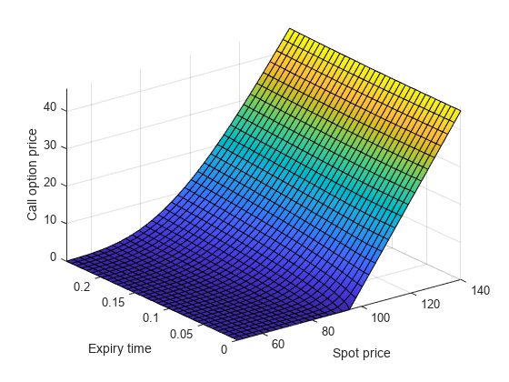
Next, suppose that for the same stock option the time to expiry changes and the day-to-day stock price is unknown. Find the price of this call option for expiry time that varies from 0 to 0.25 years, and spot price that varies from $50 to $140. Use the values for exercise rate (K), volatility (sigma), and interest rate (r) from the previous example. In this case, use the time to expiry T and day-to-day stock price S as the variable quantities.
Define the symbolic expression C to represent the call option price with T and S as the unknown variables.
syms T S

PV_K = K*exp(-r*T);
d1 = (log(S/K) + (r + sigma^2/2)*T)/(sigma*sqrt(T));
d2 = d1 - sigma*sqrt(T);
Nd1 = int(exp(-((t)^2)/2),-Inf,d1)*1/sqrt(2*pi);
Nd2 = int(exp(-((t)^2)/2),-Inf,d2)*1/sqrt(2*pi);
C = Nd1*S - Nd2*PV_K;
Plot the call option price as a function of spot price and expiry time.
fsurf(C,[50 140 0 0.25])
xlabel('Spot price')
ylabel('Expiry time')
zlabel('Call option price')
Calculate the call option price with expiry time 0.1 years and spot price $105. Use subs to substitute the values of T and S to the expression C. Return the price as a numeric result using vpa.
Csym = subs(C,[T S],[0.1 105]);
Cvpa = vpa(Csym)
Cvpa =
Find Spot Price
Consider the case where the option price is changing, and you want to know how this affects the underlying stock price. This is a problem of finding from the Black–Scholes formula given the known parameters , , , , and .
For example, after one month, the price of the same call option now trades at $15.04 with expiry time of two months. Find the spot price of the underlying stock. Create a symbolic function C(S) that represents the Black–Scholes formula with the unknown parameter S.
syms C(S) d1(S) d2(S) Nd1(S) Nd2(S)

K = 95;         % exercise price (strike price)
sigma = 0.50;   % volatility of stock
T = 2/12;       % expiry time in years
r = 0.01;       % annualized risk-free interest rate

PV_K = K*exp(-r*T);
d1(S) = (log(S/K) + (r + sigma^2/2)*T)/(sigma*sqrt(T));
d2(S) = d1 - sigma*sqrt(T);
Nd1(S) = int(exp(-((t)^2)/2),-Inf,d1)*1/sqrt(2*pi);
Nd2(S) = int(exp(-((t)^2)/2),-Inf,d2)*1/sqrt(2*pi);
C(S) = Nd1*S - Nd2*PV_K;
Use vpasolve to numerically solve for the spot price of the underlying stock. Search for solutions only in the positive numbers. The spot price of the underlying stock is $106.162.
S_Sol = vpasolve(C(S) == 15.04,S,[0 Inf])
S_Sol =
Find Implied Volatility
Consider the case where the option price is changing and you want to know what is the implied volatility. This is a problem of finding the value of from the Black–Scholes formula given the known parameters , , , , and .
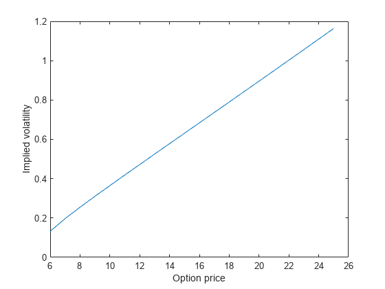
Consider the same stock option that expires in three months with an exercise price of $95. Assume that the underlying stock trades at $100, and the risk-free rate is 1% per annum. Find the implied volatility as a function of option price that ranges from $6 to $25. Create a vector for the range of the option price. Create a symbolic function C(sigma) that represents the Black–Scholes formula with the unknown parameter sigma. Use vpasolve to numerically solve for the implied volatility.
syms C(sigma) d1(sigma) d2(sigma) Nd1(sigma) Nd2(sigma)

S = 100;        % current stock price (spot price)
K = 95;         % exercise price (strike price)
T = 3/12;       % expiry time in years
r = 0.01;       % annualized risk-free interest rate
C_Range = 6:25; % range of option price
sigma_Sol = zeros(size(C_Range));

PV_K = K*exp(-r*T);
d1(sigma) = (log(S/K) + (r + sigma^2/2)*T)/(sigma*sqrt(T));
d2(sigma) = d1 - sigma*sqrt(T);
Nd1(sigma) = int(exp(-((t)^2)/2),-Inf,d1)*1/sqrt(2*pi);
Nd2(sigma) = int(exp(-((t)^2)/2),-Inf,d2)*1/sqrt(2*pi);
C(sigma) = Nd1*S - Nd2*PV_K;
for i = 1:length(C_Range)
    sigma_Sol(i) = vpasolve(C(sigma) == C_Range(i),sigma,[0 Inf]);
end
Plot the implied volatility as a function of the option price.
plot(C_Range,sigma_Sol)
xlabel('Option price')
ylabel('Implied volatility')