Generate Skidpad Test
This example shows how to simulate a skidpad test similar to events held in student competitions by Formula Student, Formula SAE, and other organizations internationally. In these, student teams build, operate, and present vehicles of their own design.
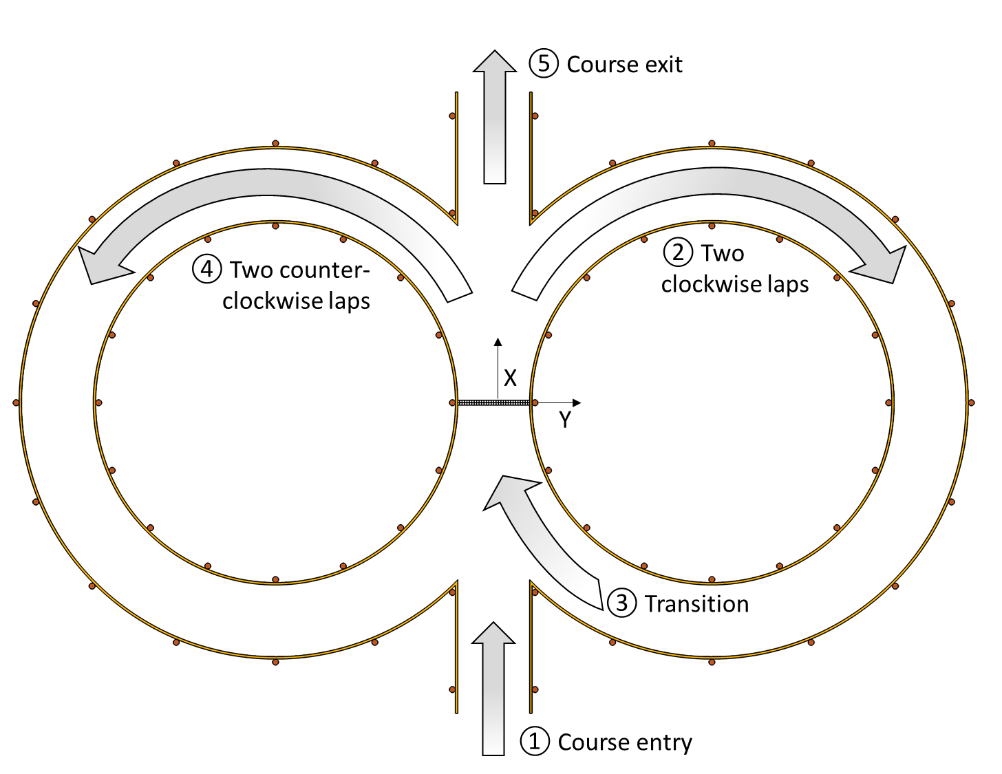
In this example, the vehicle starts from rest, then:
Accelerates to enter the course
Completes two clockwise laps
Reverses its steering direction
Completes two counterclockwise laps
Exits and brakes to a stop
Open Model
The skidpad model includes a reference path, driver, vehicle, and visualization aides. To open the model, use this command.
open_system('vdynblksskidpad');
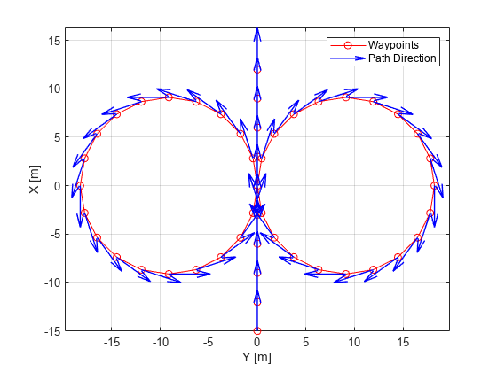
The model workspace variable TrackPoints contains the reference waypoints used to define the reference pose. You can edit or replace them with waypoints of your own. To plot the waypoints, use this code.
mdlWks = get_param('vdynblksskidpad','ModelWorkspace');
TrackPoints = evalin(mdlWks,'TrackPoints');
figure;
plot(TrackPoints(:,2),TrackPoints(:,1),'ro-');
hold on;
arrowLen = 1.5;
quiver(TrackPoints(:,2),TrackPoints(:,1), ...
    arrowLen*sin(TrackPoints(:,3)),arrowLen*cos(TrackPoints(:,3)), ...
    'b','LineWidth',1,'MaxHeadSize',arrowLen);
box on;
grid on;
xlabel('Y [m]');
ylabel('X [m]');
axis equal;
legend('Waypoints','Path Direction');
The default vehicle path follows the centerline of the course, with some X,Y points duplicated because the vehicle completes multiple laps. You can change factors such as the number of laps or scaling via the blocks found in the Skidpad Reference subsystem. You can also experiment with path points to improve lap times.
Simulate Model
To run the model and observe the vehicle completing the course, use this command.
sim('vdynblksskidpad');By default, an overhead figure depicting the reference and simulated vehicle path, and acceleration diagram are opened and updated during simulation. Lap times are estimated and displayed in order at the top level of the model via a Display block.
Modify Vehicle Type and Powertrain
You configure the Formula Student Vehicle block to use one of these variant subsystems:
Simulink Physics
Game Engine Physics
To select one of the variant subsystems, double-click the Formula Student Vehicle block and select from the Vehicle Type dropdown list or set the vehicle type programmatically using the set_param function.
Simulink Physics
The Simulink Physics variant uses a 7DOF vehicle with variant subsystems for the powertrain and final drive. By default, the powertrain variant subsystem is configured to use an ideal internal combustion engine and the final drive variant subsystem is configured to use rear wheel drive. You can set the powertrainType and finalDriveType to switch configurations. To switch to an idealized in-wheel electric vehicle with torque vectoring, set powertrainType to EV and finalDriveType to Direct. In this configuration, the model uses a set of mapped electric motors and gearboxes.
powertrainType ='EV4EM' finalDriveType =
'Direct' set_param('vdynblksskidpad/Formula Student Vehicle/Simulink Physics - 7DOF/Powertrain & Driveline/Powertrain','LabelModeActiveChoice',powertrainType); set_param('vdynblksskidpad/Formula Student Vehicle/Simulink Physics - 7DOF/Powertrain & Driveline/Final Drive','LabelModeActiveChoice',finalDriveType); if strcmp(powertrainType,'EV') set_param('vdynblksskidpad/Driver Commands/Linear Predictive Driver','shftType','Reverse, Neutral, Drive') else set_param('vdynblksskidpad/Driver Commands/Linear Predictive Driver','shftType','Scheduled') end
Run the simulation.
ev4EM = sim('vdynblksskidpad');Each of the motor's currents can be plotted as a function of time in the Simulink Data Inspector, as well as the output torques and speeds (in RPM).
plot(find(ev4EM.logsout,"BattCurr"));
plot(find(ev4EM.logsout,"MtrTrq"));
plot(find(ev4EM.logsout,"<MtrSpd>"));
Game Engine Physics
The Game Engine Physics variant subsystem has similar parameters for an internal combustion engine but uses a simulation 3D interface to configure and solve for the dynamic response of the predefined vehicle template. Given the differences in tire models and solver engines between the two settings, differences in results are to be expected. Choose your setting based on your modeling and visualization preferences.
Set vehType to Game Engine Physics to configure the model to use the game engine vehicle.
vehType = 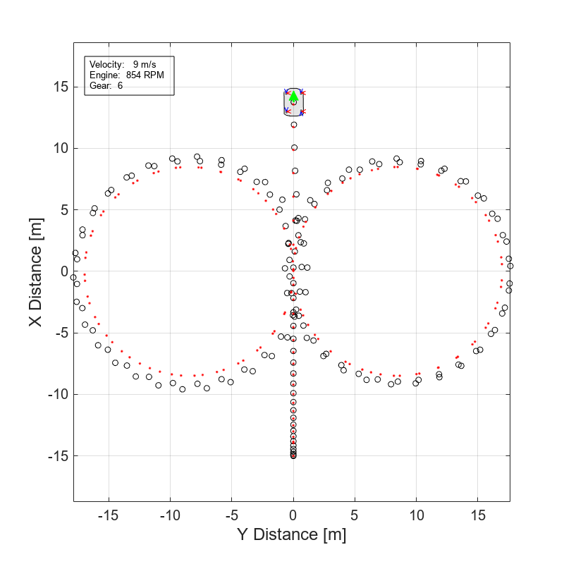 "Game Engine Physics"
Enable 3D Visualization
Before running the model in the 3D visualization environment, review the Unreal Engine Simulation Environment Requirements and Limitations.
To enable the 3D visualization, use this command.
set_param('vdynblksskidpad/Visualization/3D Visualization', ...
    'engine3D','Enabled - Simulink 3D Vehicle');
Add cones and a skidpad lane boundary texture.
set_param('vdynblksskidpad/Visualization/3D Visualization','conesOn','on');
Include tire force, vehicle and driveline annotations.
set_param('vdynblksskidpad/Visualization/3D Visualization','annotOn','on');
Run the simulation.
sim('vdynblksskidpad');You can also place cones with Simulink 3D Animation to better define the skidpad course when using the 3D visualization engine. You can adjust cone placement through the initialization script in the Simulation 3D Actor block. For more information, see Place Cones on Formula Student Skidpad Track Using Simulation 3D Animation Functions.
See Also
Simulation 3D Physics Vehicle | Simulation 3D Actor (Simulink 3D Animation)