Critically Sampled Wavelet Packet Analysis

This example shows how to obtain the wavelet packet transform of a 1-D signal. The example also demonstrates that frequency ordering is different from Paley ordering.

Save the current boundary extension mode, then set the mode to periodization.

st = dwtmode("status","nodisplay");
dwtmode("per","nodisp")

Create a signal consisting of a sine wave with a frequency of $$7\pi /8$$ radians/sample in additive white Gaussian N(0,1/4) noise. The sine wave occurs between samples 128 and 512 of the signal.

n = 0:1023;
indices = (n>127 & n<=512);
x = cos(7*pi/8*n).*indices+0.5*randn(size(n));

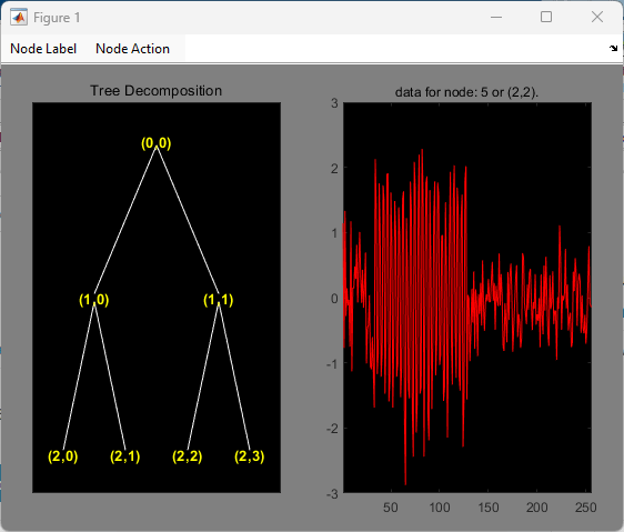
Obtain the wavelet packet transform down to level 2 using the Daubechies least asymmetric wavelet with 4 vanishing moments. Plot the wavelet packet tree.

T = wpdec(x,2,"sym4");
plot(T)

Find the Paley and frequency ordering of the terminal nodes.

[tn_pal,tn_freq] = otnodes(T)

tn_pal = 4×1

     3
     4
     5
     6

tn_freq = 4×1

     3
     4
     6
     5

tn_freq contains the vector [3 4 6 5], which shows that the highest frequency interval, $$[3\pi /4,\pi )$$, is actually node 5 in the Paley-ordered wavelet packet tree.

Click on node (2,2) in the wavelet packet tree to see that the frequency ordering correctly predicts the presence of the sine wave.

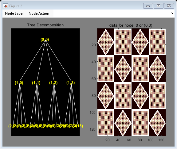
The wavelet packet transform of a 2-D image yields a quaternary wavelet packet tree. Load an example image. Use the biorthogonal B-spline wavelet with 3 vanishing moments in the reconstruction wavelet and 5 vanishing moments in the decomposition wavelet. Plot the resulting quaternary wavelet packet tree.

load tartan
T = wpdec2(X,2,"bior3.5");
plot(T)

Restore the original extension mode.

dwtmode(st,"nodisplay")

See Also

Apps

• Wavelet Signal Analyzer

Functions

• dwpt | wavedec | wavedec2

Related Topics

• Practical Introduction to Multiresolution Analysis
• Wavelet Packets: Decomposing the Details