Main Content

dwtfilterbank

Discrete wavelet transform filter bank

Description

Use dwtfilterbank to create a discrete wavelet transform (DWT) filter bank

  • Visualize wavelets and scaling functions in time and frequency.

  • Measure the 3-dB bandwidths of the wavelet and scaling functions. You can also measure energy concentration of the wavelet and scaling functions in the theoretical DWT passbands.

  • Create a DWT filter bank using your own custom filters. You can determine whether the filter bank is orthogonal or biorthogonal.

  • Determine the frame bounds of the filter bank.

Creation

Description

fb = dwtfilterbank create a discrete wavelet transform (DWT) filter bank. The default filter bank is designed for a signal with 1024 samples. The default filter bank uses the analysis (decomposition) sym4 wavelet and scaling filter with seven resolution levels.

example

fb = dwtfilterbank(Name,Value) creates a DWT filter bank fb with properties specified by one or more Name,Value pair arguments. Properties can be specified in any order as Name1,Value1,...,NameN,ValueN. Enclose each property name in quotes.

For example, fb = dwtfilterbank('SignalLength',1000,'Wavelet','bior4.4') creates a DWT filter bank for signals of length 1000 using the biorthogonal bior4.4 wavelet.

Note

You cannot change a property value of an existing filter bank. For example, if you have a filter bank fb for the sym4 wavelet, you must create a second filter bank fb2 for the coif5 wavelet. You cannot assign a different Wavelet to fb.

example

Properties

expand all

Signal length, specified as a positive integer greater than or equal to 2.

Example: 'SignalLength',768

Data Types: double

Name of wavelet used to construct the filter bank, specified as a character vector or string scalar. Wavelet is an orthogonal or biorthogonal wavelet recognized by wavemngr or 'Custom'.

To use a wavelet filter not recognized by wavemngr, set the Wavelet property to 'Custom' and specify the CustomWaveletFilter and CustomScalingFilter properties.

Example: 'Wavelet','bior4.4'

Data Types: char | string

Wavelet filter type, specified as one of 'Analysis' or 'Synthesis'. 'Analysis' uses the decomposition filters returned by wfilters. 'Synthesis' uses the reconstruction filters.

Wavelet transform level, specified as a positive integer less than or equal to floor(log2(SignalLength)). For a signal of length 1024 and the sym4 wavelet, the default level is 7.

By default the level is equal to floor(log2(SignalLength/(L-1))) where L is the length of the wavelet filter associated with Wavelet. For wavelets recognized by wavemngr, the transform level is equal to wmaxlev(SignalLength,Wavelet). If floor(log2(SignalLength/(L-1))) is less than or equal to 0, Level defaults to floor(log2(SignalLength)).

Sampling frequency in hertz, specified as a positive scalar. If unspecified, frequencies are in cycles/sample and the Nyquist frequency is ½.

Example: 'SamplingFrequency',5

Data Types: double

Custom wavelet filter coefficients, specified as a real-valued column vector or matrix. CustomWaveletFilter must be an even-length column vector for an orthogonal wavelet or a two-column matrix with an even number of rows for a biorthogonal wavelet.

This property applies only when Wavelet is set to 'Custom'.

Custom scaling filter coefficients, specified as a real-valued column vector or matrix. CustomScalingFilter must be an even-length column vector for an orthogonal wavelet or a two-column matrix with an even number of rows for a biorthogonal wavelet.

This property applies only when Wavelet is set to 'Custom'.

Object Functions

dwtpassbandsDWT filter bank passbands
filtersDWT filter bank filters
frameboundsDWT filter bank frame bounds
freqzDWT filter bank frequency responses
isBiorthogonalDetermine if DWT filter bank is biorthogonal
isOrthogonalDetermine if DWT filter bank is orthogonal
powerbwDWT filter bank power bandwidth
qfactorDWT filter bank quality factor
scalingfunctionsDWT filter bank time-domain scaling functions
waveletsDWT filter bank time-domain wavelets
waveletsupportDWT filter bank time supports

Examples

collapse all

Create a DWT filter bank using default values.

fb = dwtfilterbank
fb = 
  dwtfilterbank with properties:

                Wavelet: 'sym4'
           SignalLength: 1024
                  Level: 7
      SamplingFrequency: 1
             FilterType: 'Analysis'
    CustomWaveletFilter: []
    CustomScalingFilter: []

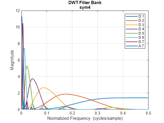
Plot the magnitude frequency responses of the wavelets and coarsest-scale scaling function. Open the plot in a separate figure window. The plot legend in the window is interactive. To hide a particular frequency response, click on its name.

freqz(fb)

Figure contains an axes object. The axes object with title DWT Filter Bank sym4, xlabel Normalized Frequency (cycles/sample), ylabel Magnitude contains 8 objects of type line. These objects represent D 1, D 2, D 3, D 4, D 5, D 6, D 7, A 7.

Obtain and plot the time-centered wavelets corresponding to the wavelet bandpass filters.

[psi,t] = wavelets(fb);
plot(t,psi')
grid on
title('Time-Centered Wavelets')
xlabel('Time')
ylabel('Magnitude')

Figure contains an axes object. The axes object with title Time-Centered Wavelets, xlabel Time, ylabel Magnitude contains 7 objects of type line.

This example shows how to create a DWT filter bank using custom biorthogonal wavelet filters.

Two pairs of analysis (decomposition) and synthesis (reconstruction) filters are associated with a biorthogonal wavelet. Each pair consists of a lowpass and highpass filter. Specify the analysis and synthesis filters for the nearly-orthogonal biorthogonal wavelets based on the Laplacian pyramid scheme of Burt and Adelson (Table 8.4 on page 283 in [1]). Hd and Gd are the lowpass and highpass decomposition filters, respectively. Hr and Gr are the lowpass and highpass reconstruction filters, respectively. Because the toolbox requires that all filters associated with a biorthogonal wavelet or an orthogonal wavelet have the same even length, prepend and append zeros to the filters.

Hd = [0 -1 5 12 5 -1 0 0]/20*sqrt(2);
Gd = [0 3 -15 -73 170 -73 -15 3]/280*sqrt(2);
Hr = [0 -3 -15 73 170 73 -15 -3]/280*sqrt(2);
Gr = [0 -1 -5 12 -5 -1 0 0]/20*sqrt(2);

Construct analysis and synthesis DWT filter banks using the biorthogonal filters. Confirm the filter banks are biorthogonal and not orthogonal.

fbAna = dwtfilterbank('Wavelet','Custom', ...
    'CustomScalingFilter',[Hd' Hr'], ...
    'CustomWaveletFilter',[Gd' Gr']);
fbSyn = dwtfilterbank('Wavelet','Custom', ...
    'CustomScalingFilter',[Hd' Hr'], ...
    'CustomWaveletFilter',[Gd' Gr'], ...
    'FilterType','Synthesis');
fprintf('fbAna: isOrthogonal = %d\tisBiorthogonal = %d\n', ...
    isOrthogonal(fbAna),isBiorthogonal(fbAna));
fbAna: isOrthogonal = 0	isBiorthogonal = 1
fprintf('fbSyn: isOrthogonal = %d\tisBiorthogonal = %d\n', ...
    isOrthogonal(fbSyn),isBiorthogonal(fbSyn ));
fbSyn: isOrthogonal = 0	isBiorthogonal = 1

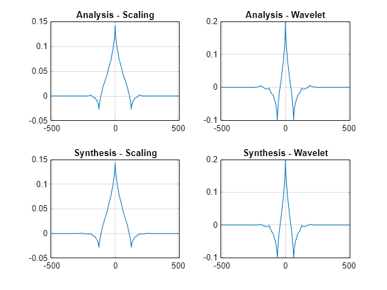
Obtain the wavelet and scaling functions of both filter banks. Plot the wavelet and scaling functions at the coarsest scales.

[fbAna_phi,t] = scalingfunctions(fbAna);
[fbAna_psi,~] = wavelets(fbAna);
[fbSyn_phi,~] = scalingfunctions(fbSyn);
[fbSyn_psi,~] = wavelets(fbSyn);
subplot(2,2,1)
plot(t,fbAna_phi(end,:))
grid on
title('Analysis - Scaling')
subplot(2,2,2)
plot(t,fbAna_psi(end,:))
grid on
title('Analysis - Wavelet')
subplot(2,2,3)
plot(t,fbSyn_phi(end,:))
grid on
title('Synthesis - Scaling')
subplot(2,2,4)
plot(t,fbSyn_psi(end,:))
grid on
title('Synthesis - Wavelet')

Figure contains 4 axes objects. Axes object 1 with title Analysis - Scaling contains an object of type line. Axes object 2 with title Analysis - Wavelet contains an object of type line. Axes object 3 with title Synthesis - Scaling contains an object of type line. Axes object 4 with title Synthesis - Wavelet contains an object of type line.

Compute the framebounds of the two filter banks. Since the filters are associated with biorthogonal wavelets, the framebounds will not equal 1.

[a1,a2] = framebounds(fbAna)
a1 = 
0.9505
a2 = 
1.0211
[b1,b2] = framebounds(fbSyn)
b1 = 
0.9800
b2 = 
1.0528

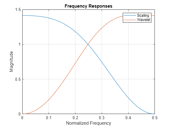
Obtain the frequency responses of the scaling and wavelets filters in the analysis filter bank. Plot up to Nyquist the magnitude frequency responses of the scaling and wavelet filters at the finest scale.

[psidft,f,phidft] = freqz(fbAna);
flen = length(f);
figure
plot(f(flen/2+1:end),abs(phidft(1,flen/2+1:end)))
hold on
plot(f(flen/2+1:end),abs(psidft(1,flen/2+1:end)))
hold off
grid on
legend('Scaling','Wavelet')
title('Frequency Responses')
xlabel('Normalized Frequency')
ylabel('Magnitude')

Figure contains an axes object. The axes object with title Frequency Responses, xlabel Normalized Frequency, ylabel Magnitude contains 2 objects of type line. These objects represent Scaling, Wavelet.

Zoom in and confirm the magnitude frequency responses at the point of intersection are not magnitude equal to 1. Plot the sum of the squared magnitudes of the frequency responses. Because the scaling (lowpass) and wavelet (highpass) filters do not form an orthogonal quadrature mirror filter pair, the sum does not equal to 2 at all frequencies.

figure
plot(f(flen/2+1:end), ...
    abs(phidft(1,flen/2+1:end)).^2+abs(psidft(1,flen/2+1:end)).^2)
grid on
title('Sum of Squared Frequency Responses')
xlabel('Normalized Frequency')
ylabel('Sum of Magnitudes')

Figure contains an axes object. The axes object with title Sum of Squared Frequency Responses, xlabel Normalized Frequency, ylabel Sum of Magnitudes contains an object of type line.

References

[1] Daubechies, I. Ten Lectures on Wavelets. CBMS-NSF Regional Conference Series in Applied Mathematics. Philadelphia, PA: Society for Industrial and Applied Mathematics, 1992.

Version History

Introduced in R2018a