Main Content

scal2frq

Scale to frequency

Description

frq = scal2frq(A,wname,delta) returns the pseudo-frequencies corresponding to the scales given by A and the wavelet specified by wname and the sampling period delta. The output frq is real-valued and has the same dimensions as A.

example

frq = scal2frq(A,wname) is equivalent to frq = scal2frq(A,wname,1).

Examples

collapse all

This example shows how the pseudo-frequency changes as you double the scale.

Construct a vector of scales with 10 voices per octave over five octaves.

vpo = 10;
no = 5;
a0 = 2^(1/vpo);
ind = 0:vpo*no;
sc = a0.^ind;

Verify that the range of scales covers five octaves.

log2(max(sc)/min(sc))
ans = 
5.0000

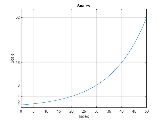
If you plot the scales, you can use a data cursor to confirm that the scale at index n+10 is twice the scale at index n. Set the y-ticks to mark each octave.

plot(ind,sc)
title('Scales')
xlabel('Index')
ylabel('Scale')
grid on
set(gca,'YTick',2.^(0:5))

Figure contains an axes object. The axes object with title Scales, xlabel Index, ylabel Scale contains an object of type line.

Convert the scales to pseudo-frequencies for the real-valued Morlet wavelet. First, assume the sampling period is 1. Since there are 10 voices per octave, display every tenth row in the table. Observe that for each doubling of the scale, the pseudo-frequency is cut in half.

pf = scal2frq(sc,"morl");
T = [sc(:) pf(:)];
T = array2table(T, ...
    'VariableNames',{'Scale','Pseudo-Frequency'});
disp(T(1:10:end,:))
    Scale    Pseudo-Frequency
    _____    ________________

      1            0.8125    
      2           0.40625    
      4           0.20313    
      8           0.10156    
     16          0.050781    
     32          0.025391    

Assume that data is sampled at 100 Hz. Construct a table with the scales, the corresponding pseudo-frequencies, and periods. Display every tenth row in the table.

Fs = 100;
DT = 1/Fs;
pf = scal2frq(sc,"morl",DT);
T = [sc(:)/Fs pf(:) 1./pf(:)];
T = array2table(T, ...
    'VariableNames',{'Scale','Pseudo-Frequency','Period'});
T(1:vpo:end,:)
ans=6×3 table
    Scale    Pseudo-Frequency     Period 
    _____    ________________    ________

    0.01           81.25         0.012308
    0.02          40.625         0.024615
    0.04          20.313         0.049231
    0.08          10.156         0.098462
    0.16          5.0781          0.19692
    0.32          2.5391          0.39385

Note the presence of the Δt=1Fs factor in scal2frq. This is necessary in order to achieve the proper scale-to-frequency conversion. The Δt is needed to adjust the raw scales properly. For example, with:

f = scal2frq(1,'morl',0.01);

You are really asking what happens to the center frequency of the mother Morlet wavelet, if you dilate the wavelet by 0.01. In other words, what is the effect on the center frequency if instead of ψ(t), you look at ψ(t/0.01). The Δt provides the correct adjustment factor on the scales.

You could have obtained the same results by first converting the scales to their adjusted sizes and then using scal2frq without specifying Δt.

scadjusted = sc.*0.01;
pf2 = scal2frq(scadjusted,'morl');
max(pf-pf2)
ans = 
0

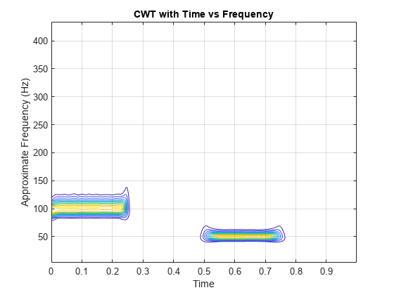
The example shows how to create a contour plot of the CWT using approximate frequencies in Hz.

Create a signal consisting of two sine waves with disjoint support in additive noise. Assume the signal is sampled at 1 kHz.

Fs = 1000;
t = 0:1/Fs:1-1/Fs;
x = 1.5*cos(2*pi*100*t).*(t<0.25)+1.5*cos(2*pi*50*t).*(t>0.5 & t<=0.75);
x = x+0.05*randn(size(t));

Obtain the CWT of the input signal and plot the result.

[cfs,f] = cwt(x,Fs);
contour(t,f,abs(cfs).^2); 
axis tight;
grid on;
xlabel('Time');
ylabel('Approximate Frequency (Hz)');
title('CWT with Time vs Frequency');

Figure contains an axes object. The axes object with title CWT with Time vs Frequency, xlabel Time, ylabel Approximate Frequency (Hz) contains an object of type contour.

Input Arguments

collapse all

Scales, specified as a positive real-valued vector.

Wavelet, specified as a character vector or string scalar. See wavefun for more information.

Sampling period, specified as a real-valued scalar.

Example: pf = scal2frq([1:5],"db4",0.01)

More About

collapse all

Pseudo-Frequencies

There is only an approximate answer for the relationship between scale and frequency.

In wavelet analysis, the way to relate scale to frequency is to determine the center frequency of the wavelet, Fc, and use the following relationship:

Fa=Fca

where

  • a is a scale.

  • Fc is the center frequency of the wavelet in Hz.

  • Fa is the pseudo-frequency corresponding to the scale a, in Hz.

The idea is to associate with a given wavelet a purely periodic signal of frequency Fc. The frequency maximizing the Fourier transform of the wavelet modulus is Fc. The centfrq function computes the center frequency for a specified wavelet. From the above relationship, it can be seen that scale is inversely proportional to pseudo-frequency. For example, if the scale increases, the wavelet becomes more spread out, resulting in a lower pseudo-frequency.

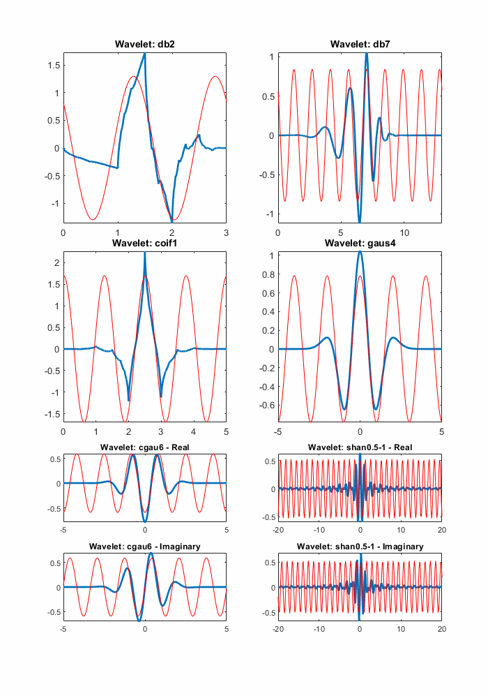
Some examples of the correspondence between the center frequency and the wavelet are shown in the following figure.

Center Frequencies for Real and Complex Wavelets

As you can see, the center frequency-based approximation (red) captures the main wavelet oscillations (blue). The center frequency is a convenient and simple characterization of the dominant frequency of the wavelet.

References

[1] Abry, P. Ondelettes et turbulence. Multirésolutions, algorithmes de décomposition, invariance d'échelles et signaux de pression. Diderot, Editeurs des sciences et des arts, Paris, 1997.

Version History

Introduced before R2006a

See Also