filterbank
Syntax
Description
[
returns the spin-up and spin-down frequency wavelets, psifup,psifdown,phiffr,frequencymeta] = filterbank(jtfn,FilterBank="frequency")psifup and
psifdown respectively, the frequency lowpass filter
phiffr, and the metadata frequencymeta for the
frequency filters in the JTFS network.
The syntax filterbank(jtfn,FilterBank="time") is equivalent to
filterbank(jtfn).
Examples
Create a JTFS network with the energy correct filters option set to false. Specify quality factors of 9 and 2 for the first-order and second-order time wavelet filter banks, respectively.
jtfn = timeFrequencyScattering(EnergyCorrectFilters=false, ...
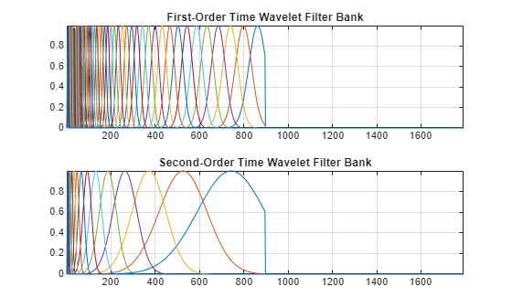
TimeQualityFactors=[9 2]);Obtain the filters in the first- and second-order time wavelet filter banks and their metadata. Plot the filters. Because the wavelets are analytic, their Fourier transforms are supported only on the positive real axis.
[psi1f,psi2f,phift,timemeta] = filterbank(jtfn);
tiledlayout(2,1)
nexttile
plot(psi1f)
grid on
axis tight
title("First-Order Time Wavelet Filter Bank")
nexttile
plot(psi2f)
grid on
axis tight
title("Second-Order Time Wavelet Filter Bank")
Inspect the size and metadata for the first-order time wavelet filter bank. The wavelet filters are arranged columnwise and in order of decreasing center frequency. The th table row describes the th filter.
size(psi1f)
ans = 1×2

        1792          50
timemeta{1}ans=50×6 table
xi sigma isCQT log2dsfactor peakidx bwidx
_______ _________ _____ ____________ _______ __________
0.48076 0.022225 1 0 863 757 897
0.44512 0.020578 1 0 799 701 896
0.41212 0.019053 1 0 740 646 833
0.38158 0.01764 1 0 685 598 771
0.35329 0.016333 1 0 634 553 714
0.3271 0.015122 1 0 587 512 661
0.30286 0.014001 1 0 544 475 613
0.28041 0.012963 1 0 503 440 567
0.25962 0.012002 1 0 466 407 525
0.24038 0.011113 1 0 432 377 486
0.22256 0.010289 1 0 400 349 450
0.20606 0.0095263 1 1 370 324 417
0.19079 0.0088202 1 1 343 300 386
0.17665 0.0081664 1 1 318 278 358
0.16355 0.007561 1 1 294 257 331
0.15143 0.0070006 1 1 272 237 306
⋮
Choose a time filter bank. From its metadata, obtain the filter center frequencies and the logical values indicating if a center frequency is logarithmically spaced.
whichFB = 1;
centerFrq = timemeta{whichFB}.xi;
isCQT = timemeta{whichFB}.isCQT;
Compute the ratios of consecutive center frequencies that are logarithmically spaced. Confirm the ratios are equal to , where is the quality factor of the filter bank.
qualityFactor = jtfn.TimeQualityFactors(whichFB);
isLogSpaced = find(isCQT);
cf = centerFrq(isLogSpaced);
cfRatio = cf(2:end)./cf(1:end-1);
[min(cfRatio) max(cfRatio) 2^(-1/qualityFactor)]
ans = 1×3

    0.9259    0.9259    0.9259
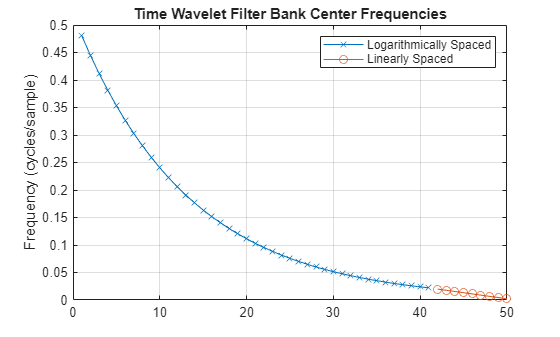
Plot on a linear scale with a cross marker the center frequencies that are logarithmically spaced. Then plot with a circle marker the center frequencies that are linearly spaced.
figure
plot(isLogSpaced,cf,'x-')
hold on
isNotLogSpaced = find(~isCQT);
plot(isNotLogSpaced,centerFrq(isNotLogSpaced),'o-')
hold off
grid on
legend("Logarithmically Spaced","Linearly Spaced")
title("Time Wavelet Filter Bank Center Frequencies")
ylabel("Frequency (cycles/sample)")
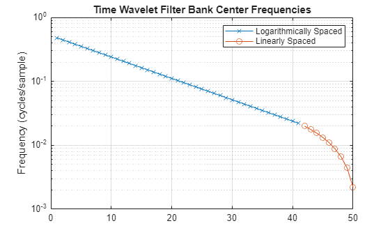
Make the same plot, but this time on a logarithmic scale.
figure
semilogy(isLogSpaced,centerFrq(isLogSpaced),'x-')
hold on
semilogy(isNotLogSpaced,centerFrq(isNotLogSpaced),'o-')
hold off
grid on
legend("Logarithmically Spaced","Linearly Spaced")
title("Time Wavelet Filter Bank Center Frequencies")
ylabel("Frequency (cycles/sample)")
Create a JTFS network with the energy correct filters option set to false. Specify a frequency quality factor of 3.
jtfn = timeFrequencyScattering(EnergyCorrectFilters=false, ...
    FrequencyQualityFactor=3)
jtfn =
timeFrequencyScattering with properties:
SignalLength: 1024
NumFrequencyOctaves: 3
FrequencyInvarianceScale: 8
FrequencyQualityFactor: 3
TimeInvarianceScale: 128
TimeQualityFactors: [8 1]
TimeMaxPaddingFactor: 2
NumTimeOctaves: [7 7]
FilterDataType: 'double'
FrequencyMaxPaddingFactor: 2
EnergyCorrectFilters: 0
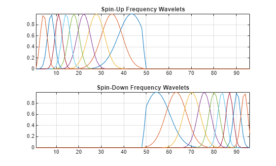
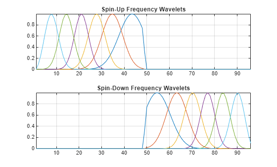
Obtain the spin-up and spin-down frequency wavelets and their metadata. Plot the wavelets.
[psifup,psifdown,phiffr,frequencymeta] = filterbank(jtfn, ...
    FilterBank="frequency");
tiledlayout(2,1)
nexttile
plot(psifup)
grid on
title("Spin-Up Frequency Wavelets")
axis tight
nexttile
plot(psifdown)
title("Spin-Down Frequency Wavelets")
grid on
axis tight
Inspect the metadata. The metadata is listed in order of decreasing center frequency, first for the spin-up wavelets, and then the spin-down wavelets.
frequencymeta
frequencymeta=18×7 table
       xi        sigma      isCQT    log2dsfactor    spin    peakidx     bwidx
    ________    ________    _____    ____________    ____    _______    ________

     0.44249    0.061128      1           0            1       43       28    49
     0.35121    0.048518      1           0            1       35       22    47
     0.27875    0.038508      1           0            1       28       18    38
     0.22125    0.030564      1           0            1       22       14    30
      0.1756    0.024259      1           1            1       18       12    24
     0.13938    0.019254      1           1            1       14       10    19
     0.10453     0.01625      0           1            1       11        7    15
    0.069688     0.01625      0           2            1        8        4    12
    0.034844     0.01625      0           2            1        4        2     8
    -0.44249    0.061128      1           0           -1       55       49    70
    -0.35121    0.048518      1           0           -1       63       51    76
    -0.27875    0.038508      1           0           -1       70       60    80
    -0.22125    0.030564      1           0           -1       76       68    84
     -0.1756    0.024259      1           1           -1       80       74    86
    -0.13938    0.019254      1           1           -1       84       79    88
    -0.10453     0.01625      0           1           -1       87       83    91
      ⋮
Obtain the center quefrencies of the spin-up wavelets and the logical value indicating if a center quefrency is logarithmically spaced.
numRows = size(frequencymeta,1);
centerQf = frequencymeta.xi(1:numRows/2);
isCQT = frequencymeta.isCQT(1:numRows/2);
Compute the ratios of consecutive center quefrencies that are logarithmically spaced. Confirm the ratios are equal to , where is the quality factor of the filter bank.
qualityFactor = jtfn.FrequencyQualityFactor;
isLogSpaced = find(isCQT);
cf = centerQf(isLogSpaced);
cfRatio = cf(2:end)./cf(1:end-1);
[min(cfRatio) max(cfRatio) 2^(-1/qualityFactor)]
ans = 1×3

    0.7937    0.7937    0.7937
By default, the number of frequency octaves is 3. Create a second network identical to the first, but instead set the number of frequency octaves to 2. Obtain the frequency wavelets and their metadata. Plot the spin-up and spin-down wavelets. The length and number of frequency wavelets is less than those in the original JTFS network.
jtfn2 = timeFrequencyScattering(EnergyCorrectFilters=false, ...
    FrequencyQualityFactor=3, ...
    NumFrequencyOctaves=2);
[psifup2,psifdown2,~,frequencymeta2] = filterbank(jtfn2, ...
    FilterBank="frequency");
tiledlayout(2,1)
nexttile
plot(psifup2)
grid on
title("Spin-Up Frequency Wavelets")
axis tight
nexttile
plot(psifdown2)
title("Spin-Down Frequency Wavelets")
grid on
axis tight
Input Arguments
Output Arguments
Version History
Introduced in R2024b