Main Content

timeFrequencyScattering

Joint time-frequency scattering

Since R2024b

    Description

    Use timeFrequencyScattering to create a joint time-frequency scattering network using Morlet wavelets.

    Creation

    Description

    jtfn = timeFrequencyScattering creates a joint time-frequency scattering (JTFS) network with default property values.

    example

    jtfn = timeFrequencyScattering(Name=Value) sets properties using one or more name-value arguments. For example, jtfn = timeFrequencyScattering(FrequencyQualityFactor=2) creates a network that uses two frequential wavelet filters per octave. You can set properties in any order.

    Properties become read-only after you create the network.

    Properties

    expand all

    Network

    Signal length in samples, specified as a positive integer greater than or equal to 16.

    • If the input to the scattering transform is a row vector, SignalLength must match the number of columns in the input data.

    • If the input to the scattering transform is a column vector, matrix, or 3-D array, SignalLength must match the number of rows in the input data.

    For more information, see scatteringTransform and scatteringFeatures.

    To set this property, use the corresponding name-value argument when you create the timeFrequencyScattering object. After you create a timeFrequencyScattering object, this property is read-only.

    Data Types: single | double

    Filter data type, specified as "double" or "single". The network stores the filters in the specified type. When applying the filters to data, the network follows MATLAB® rules. For more information, see Arithmetic Operations on Floating-Point Numbers.

    To set this property, use the corresponding name-value argument when you create the timeFrequencyScattering object. After you create a timeFrequencyScattering object, this property is read-only.

    Energy correct filters option, specified as a numeric or logical 1 (true) or 0 (false). If you set this option to true, the network corrects the analytic time filters so that the Littlewood-Paley sum is approximately 2 from 0 to the Nyquist frequency. The frequency filters approximate 1. When you view the filters using filterbank, the filter peaks are not equal. For more information, see littlewoodPaleySum and Proposition 2.1 in [3].

    To set this property, use the corresponding name-value argument when you create the timeFrequencyScattering object. After you create a timeFrequencyScattering object, this property is read-only.

    Data Types: logical

    Time Wavelet Filters

    Time invariance scale in samples, specified as a positive integer. TimeInvarianceScale specifies the time translation invariance of the scattering transform. By default, TimeInvarianceScale is equal to 2^J, where J is the number of time octaves in the first-order time wavelet filter bank. TimeInvarianceScale cannot exceed SignalLength rounded up to the next power of 2.

    To set this property, use the corresponding name-value argument when you create the timeFrequencyScattering object. After you create a timeFrequencyScattering object, this property is read-only.

    Data Types: single | double

    Quality factors for the time wavelet filter banks, specified as a positive integer or a two-element vector of positive integers between 1 and 24. The second element must be less than or equal to the first element. A quality factor is the number of time wavelet filters per octave.

    timeFrequencyScattering discretizes the wavelet center frequencies down to the invariant scale in a geometric progression with the common ratio 2–1/Q, where Q is the quality factor of the filter bank. Frequencies lower than the invariant scale are linearly spaced with scale held constant so that the invariant is not exceeded.

    If you specify TimeQualityFactors as an integer, by default the second element is 1.

    To set this property, use the corresponding name-value argument when you create the timeFrequencyScattering object. After you create a timeFrequencyScattering object, this property is read-only.

    Example: timeFrequencyScattering(TimeQualityFactors=[6 2]) specifies a JTFS network with quality factors of 6 and 2 in the first- and second-order time wavelet filter banks, respectively.

    Data Types: single | double

    Number of octaves for time wavelets, specified as a positive integer or a two-element vector of positive integers. Both values of NumTimeOctaves must be greater than 2 and less than or equal to ceil(log2(SignalLength)). By default, NumTimeOctaves is [NTO NTO], where NTO = max(2,ceil(log2(SignalLength))-3).

    NumTimeOctaves together with TimeQualityFactors determine the number of time wavelets in each filter bank. There are approximately Q×J logarithmically-spaced wavelets, where Q is an element of TimeQualityFactors and J is the corresponding element in NumTimeOctaves.

    Setting NumTimeOctaves to N is equivalent to setting NumTimeOctaves to [N N].

    To set this property, use the corresponding name-value argument when you create the timeFrequencyScattering object. After you create a timeFrequencyScattering object, this property is read-only.

    Example: timeFrequencyScattering(NumTimeOctaves=[6 4]) specifies six and four octaves for the first- and second-order time filter banks, respectively.

    Data Types: single | double

    Base-2 time maximum padding factor, specified as 0, 1, or 2. The network uses TimeMaxPaddingFactor as follows:

    1. The network determines empirically the length to pad the lowest-frequency wavelets and scaling function so that:

      • The wavelet and scaling filters decay properly.

      • The filter length is an even multiple of 2^floor(log2(T)), where T is the time invariance scale. This ensures the filters can be downsampled by 2^floor(log2(T)).

      This length is called the ideal pad.

    2. The network pads the filters by the minimum of the ideal pad and 2^(ceil(log2(SignalLength))+TimeMaxPaddingFactor). These are the filters the network uses.

    If the ideal pad is more than twice the length derived from TimeMaxPaddingFactor, the network issues a warning message. To compare the filter decay in both sets of filters, use the filterpadding function.

    To set this property, use the corresponding name-value argument when you create the timeFrequencyScattering object. After you create a timeFrequencyScattering object, this property is read-only.

    Frequency Wavelet Filters

    Frequency invariance scale in samples, specified as a positive integer.

    When timeFrequencyScattering creates the network, the function determines the number of first-order time wavelet filter paths to each second-order time wavelet filter. If FrequencyInvarianceScale is greater than the maximum number of paths to a second-order filter, timeFrequencyScattering truncates FrequencyInvarianceScale to that value before returning the network. For more information, see numFirst2SecondFilterBank.

    To set this property, use the corresponding name-value argument when you create the timeFrequencyScattering object. After you create a timeFrequencyScattering object, this property is read-only.

    Data Types: single | double

    Quality factor for the frequential wavelet filter bank, specified as a positive integer between 1 and 24. A quality factor is the number of frequential wavelet filters per octave.

    timeFrequencyScattering discretizes the wavelet center quefrencies down to the invariant scale in a geometric progression with the common ratio 2–1/Q, where Q is the quality factor of the filter bank. Quefrencies lower than the invariant scale are linearly spaced with scale held constant so that the invariant is not exceeded.

    To set this property, use the corresponding name-value argument when you create the timeFrequencyScattering object. After you create a timeFrequencyScattering object, this property is read-only.

    Data Types: single | double

    Number of octaves for frequential wavelets, specified as a positive integer greater than or equal to 2.

    The default value of NumFrequencyOctaves depends on the maximum number of first-order time wavelet filter paths to a second-order time wavelet filter. When timeFrequencyScattering creates the network, the function sets the default value to max(2,ceil(log2(MNP)-3)), where MNP is the maximum number of first-order time wavelet filter paths to a second-order time wavelet filter. If you specify a NumFrequencyOctaves value that is greater than ceil(log2(MNP)), then timeFrequencyScattering truncates NumFrequencyOctaves to that value before returning the network. For more information, see numFirst2SecondFilterBank.

    NumFrequencyOctaves together with FrequencyQualityFactor determines the number of frequential wavelets. There are approximately Qfr×Jfr logarithmically-spaced wavelets, where Qfr is FrequencyQualityFactor and Jfr is NumFrequencyOctaves.

    To set this property, use the corresponding name-value argument when you create the timeFrequencyScattering object. After you create a timeFrequencyScattering object, this property is read-only.

    Data Types: single | double

    Base-2 frequency maximum padding factor, specified as 0, 1, or 2. The network uses FrequencyMaxPaddingFactor as follows:

    1. The network determines empirically the length to pad the lowest-frequency wavelets and scaling function so that:

      • The wavelet and scaling filters decay properly.

      • The filter length is an even multiple of 2^floor(log2(F)), where F is the frequency invariance scale. This ensures the filters can be downsampled by 2^floor(log2(F)).

      This length is called the ideal pad.

    2. The network pads the filters by the minimum of the ideal pad and 2^(ceil(log2(MNP))+FrequencyMaxPaddingFactor), where MNP is the maximum number of first-order time wavelet filter paths to a second-order time wavelet filter. These are the filters the network uses.

    If the ideal pad is more than twice the length derived from FrequencyMaxPaddingFactor, the network issues a warning message. To compare the filter decay in both sets of filters, use the filterpadding function.

    To set this property, use the corresponding name-value argument when you create the timeFrequencyScattering object. After you create a timeFrequencyScattering object, this property is read-only.

    Object Functions

    scatteringTransformWavelet joint time-frequency scattering transform
    scatteringFeaturesJoint time-frequency scattering feature tensor
    filterbankJoint time-frequency scattering filter bank
    filterpaddingJoint time-frequency scattering filter padding
    scattergramVisualize joint time-frequency scattering coefficients
    littlewoodPaleySumLittlewood-Paley sum for JTFS filters
    numFirst2SecondFilterBankNumber of paths from first- to second-order time wavelet filter bank in joint time-frequency scattering network

    Examples

    collapse all

    Create a joint time-frequency scattering network with default values.

    jtfn = timeFrequencyScattering
    jtfn = 
      timeFrequencyScattering with properties:
    
                     SignalLength: 1024
              NumFrequencyOctaves: 3
         FrequencyInvarianceScale: 8
           FrequencyQualityFactor: 1
              TimeInvarianceScale: 128
               TimeQualityFactors: [8 1]
             TimeMaxPaddingFactor: 2
                   NumTimeOctaves: [7 7]
                   FilterDataType: 'double'
        FrequencyMaxPaddingFactor: 2
             EnergyCorrectFilters: 1


    Use the filterbank object function to obtain the first- and second-order time wavelet filter banks, and the time lowpass filter. Then obtain the spin-up and spin-down wavelets, and the frequency lowpass filter.

    [psi1f,psi2f,phift] = filterbank(jtfn);
    [psiffrup,psiffrdn,phiffr] = filterbank(jtfn,FilterBank="frequency");

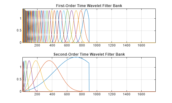
    Plot the wavelet filter banks.

    tiledlayout(2,1)
    nexttile
    plot(psi1f)
    grid on
    axis tight
    title("First-Order Time Wavelet Filter Bank")
    nexttile
    plot(psi2f)
    grid on
    axis tight
    title("Second-Order Time Wavelet Filter Bank")

    Figure contains 2 axes objects. Axes object 1 with title First-Order Time Wavelet Filter Bank contains 45 objects of type line. Axes object 2 with title Second-Order Time Wavelet Filter Bank contains 9 objects of type line.

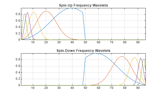
    Plot the spin-up and spin-down wavelets.

    tiledlayout(2,1)
    nexttile
    plot(psiffrup)
    grid on
    title('Spin-Up Frequency Wavelets')
    axis tight
    nexttile
    plot(psiffrdn)
    title('Spin-Down Frequency Wavelets')
    grid on
    axis tight

    Figure contains 2 axes objects. Axes object 1 with title Spin-Up Frequency Wavelets contains 5 objects of type line. Axes object 2 with title Spin-Down Frequency Wavelets contains 5 objects of type line.

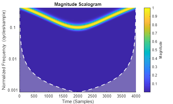
    Load the quadratic chirp signal. Visualize its continuous wavelet transform.

    load quadchirp
    cwt(quadchirp)

    Figure contains an axes object. The axes object with title Magnitude Scalogram, xlabel Time (Samples), ylabel Normalized Frequency (cycles/sample) contains 3 objects of type image, line, area.

    Create a joint time-frequency scattering network appropriate for the signal. Specify a time invariance scale of 32 samples and a quality factor of 16 for the first-order time wavelet filter bank. For the frequency wavelet filter bank, specify 2 octaves and an invariance scale of 2. To reduce memory requirements, set the filter data type to single precision.

    len = length(quadchirp);
    jtfn = timeFrequencyScattering(SignalLength=len, ...
        FilterDataType="single", ...
        TimeInvarianceScale=32, ...
        TimeQualityFactor=16, ...
        NumFrequencyOctaves=2, ...
        FrequencyInvarianceScale=2);

    Obtain the JTFS transform of the signal.

    [outCFS,outMETA] = scatteringTransform(jtfn,quadchirp);

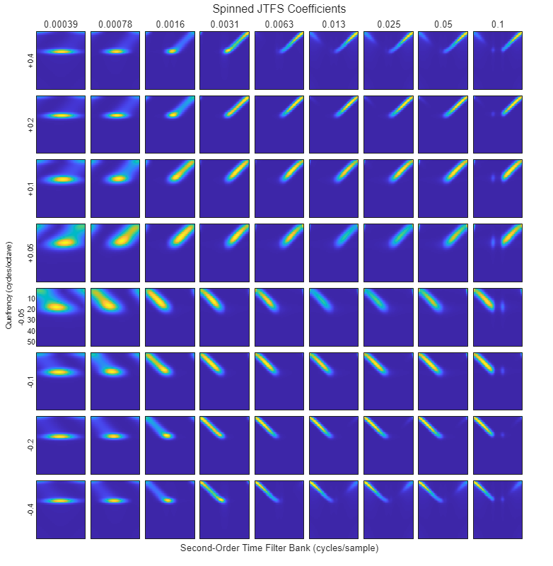
    Visual the spin-up and spin-down JTFS coefficients. The spin-up coefficients preferentially localize the up-chirp while the spin-down coefficients preferentially localize the down-chirp.

    scattergram(jtfn,outCFS,outMETA)

    Figure contains 72 axes objects. Axes object 1 with xlabel 0.1 contains an object of type image. Axes object 2 contains an object of type image. Axes object 3 contains an object of type image. Axes object 4 contains an object of type image. Axes object 5 with xlabel 0.05 contains an object of type image. Axes object 6 contains an object of type image. Axes object 7 contains an object of type image. Axes object 8 contains an object of type image. Axes object 9 with xlabel 0.025 contains an object of type image. Axes object 10 contains an object of type image. Axes object 11 contains an object of type image. Axes object 12 contains an object of type image. Axes object 13 with xlabel 0.013 contains an object of type image. Axes object 14 contains an object of type image. Axes object 15 contains an object of type image. Axes object 16 contains an object of type image. Axes object 17 with xlabel 0.0063 contains an object of type image. Axes object 18 contains an object of type image. Axes object 19 contains an object of type image. Axes object 20 contains an object of type image. Axes object 21 with xlabel 0.0031 contains an object of type image. Axes object 22 contains an object of type image. Axes object 23 contains an object of type image. Axes object 24 contains an object of type image. Axes object 25 with xlabel 0.0016 contains an object of type image. Axes object 26 contains an object of type image. Axes object 27 contains an object of type image. Axes object 28 contains an object of type image. Axes object 29 with xlabel 0.00078 contains an object of type image. Axes object 30 contains an object of type image. Axes object 31 contains an object of type image. Axes object 32 contains an object of type image. Axes object 33 with xlabel 0.00039, ylabel +0.4 contains an object of type image. Axes object 34 with ylabel +0.2 contains an object of type image. Axes object 35 with ylabel +0.1 contains an object of type image. Axes object 36 with ylabel +0.05 contains an object of type image. Axes object 37 contains an object of type image. Axes object 38 contains an object of type image. Axes object 39 contains an object of type image. Axes object 40 contains an object of type image. Axes object 41 contains an object of type image. Axes object 42 contains an object of type image. Axes object 43 contains an object of type image. Axes object 44 contains an object of type image. Axes object 45 contains an object of type image. Axes object 46 contains an object of type image. Axes object 47 contains an object of type image. Axes object 48 contains an object of type image. Axes object 49 contains an object of type image. Axes object 50 contains an object of type image. Axes object 51 contains an object of type image. Axes object 52 contains an object of type image. Axes object 53 contains an object of type image. Axes object 54 contains an object of type image. Axes object 55 contains an object of type image. Axes object 56 contains an object of type image. Axes object 57 contains an object of type image. Axes object 58 contains an object of type image. Axes object 59 contains an object of type image. Axes object 60 contains an object of type image. Axes object 61 contains an object of type image. Axes object 62 contains an object of type image. Axes object 63 contains an object of type image. Axes object 64 contains an object of type image. Axes object 65 contains an object of type image. Axes object 66 contains an object of type image. Axes object 67 contains an object of type image. Axes object 68 contains an object of type image. Axes object 69 with ylabel -0.4 contains an object of type image. Axes object 70 with ylabel -0.2 contains an object of type image. Axes object 71 with ylabel -0.1 contains an object of type image. Axes object 72 with ylabel -0.05 contains an object of type image.

    Tips

    • A large percentage of the computational burden of the JTFS algorithm comes from the element-wise multiplications, Fourier transforms, and inverse Fourier transforms. If you find the empirically determined filter lengths too long, consider setting TimeMaxPaddingFactor and FrequencyMaxPaddingFactor to 0 or 1. Depending on the padding factors, you might see a warning at object construction. To diagnose whether the reduced padding length is adequate given your network specifications, use filterpadding.

    References

    [1] Andén, Joakim, Vincent Lostanlen, and Stéphane Mallat. “Joint Time–Frequency Scattering.” IEEE Transactions on Signal Processing 67, no. 14 (July 15, 2019): 3704–18. https://doi.org/10.1109/TSP.2019.2918992

    [2] Lostanlen, Vincent, Christian El-Hajj, Mathias Rossignol, Grégoire Lafay, Joakim Andén, and Mathieu Lagrange. “Time–Frequency Scattering Accurately Models Auditory Similarities between Instrumental Playing Techniques.” EURASIP Journal on Audio, Speech, and Music Processing 2021, no. 1 (December 2021): 3. https://doi.org/10.1186/s13636-020-00187-z

    [3] Mallat, Stéphane. “Group Invariant Scattering.” Communications on Pure and Applied Mathematics 65, no. 10 (October 2012): 1331–98. https://doi.org/10.1002/cpa.21413

    Extended Capabilities

    Version History

    Introduced in R2024b