Wavelet Scattering
A wavelet scattering network enables you to derive, with minimal configuration, low-variance features from real-valued time series and image data for use in machine learning and deep learning applications. The features are insensitive to translations of the input on an invariance scale that you define and are continuous with respect to deformations. In the 2-D case, features are also insensitive to rotations. The scattering network uses predefined wavelet and scaling filters.
Mallat, with Bruna and Andén, pioneered the creation of a mathematical framework for studying convolutional neural architectures [2][3][4][5]. Andén and Lostanlen developed efficient algorithms for wavelet scattering of 1-D signals [4] [6]. Oyallon developed efficient algorithms for 2-D scattering [7]. Andén, Lostanlen, and Oyallon are major contributors to the ScatNet [10] and Kymatio [11] software for computing scattering transforms.
Mallat and others characterized three properties that deep learning architectures possess for extracting useful features from data:
Multiscale contractions
Linearization of hierarchical symmetries
Sparse representations
The wavelet scattering network exhibits all these properties. Wavelet transforms linearize small deformations such as dilations by separating the variations across different scales. For many natural signals, the wavelet transform also provides a sparse representation. By combining wavelet transforms with other features of the scattering network described below, the scattering transform produces data representations that minimize differences within a class while preserving discriminability across classes. An important distinction between the scattering transform and deep learning networks is that the filters are defined a priori as opposed to being learned. Because the scattering transform is not required to learn the filter responses, you can often use scattering successfully in situations where there is a shortage of training data.
Wavelet Scattering Transform
A wavelet scattering transform processes data in stages. The output of one stage becomes input for the next stage. Each stage consists of three operations.

The zeroth-order scattering coefficients are computed by simple averaging of the input. Here is a tree view of the algorithm:

The are wavelets, is the scaling function, and is the input data. In the case of image data, for each , there are a number of user-specified rotations of the wavelet. A sequence of edges from the root to a node is referred to as a path. The tree nodes are the scalogram coefficients. The scattering coefficients are the scalogram coefficients convolved with the scaling function . The set of scattering coefficients are the low-variance features derived from the data. Convolution with the scaling function is lowpass filtering and information is lost. However, the information is recovered when computing the coefficients in the next stage.
To extract features from the data, first use waveletScattering (for time series) or waveletScattering2 (for image data) to create and configure the network.
Parameters you set include the size of invariance scale, the number of filter banks, and
the number of wavelets per octave in each filter bank. In waveletScattering2 you can also set the number of rotations per wavelet.
To derive features from time series, use the waveletScattering object
functions scatteringTransform or featureMatrix. To derive features from image data, use the
waveletScattering2 object functions scatteringTransform or featureMatrix.
The scattering transform generates features in an iterative fashion. First, you convolve the data with the scaling function, to obtain S[0], the zeroth-order scattering coefficients. Next, proceed as follows:
Take the wavelet transform of the input data with each wavelet filter in the first filter bank.
Take the modulus of each of the filtered outputs. The nodes are the scalogram, U[1].
Average each of the moduli with the scaling filter. The results are the first-order scattering coefficients, S[1].
Repeat the process at every node.
The scatteringTransform function returns the scattering and
scalogram coefficients. The featureMatrix function returns the
scattering features. Both outputs can be made easily consumable by learning algorithms,
as demonstrated in Wavelet Time Scattering for ECG Signal Classification or Texture Classification with Wavelet Image Scattering.
Invariance Scale
The scaling filter plays a crucial role in the wavelet scattering network. When you create a wavelet scattering network, you specify the invariance scale. The network is invariant to translations up to the invariance scale. The support of the scaling function determines the size of the invariant in time or space.
Time Invariance
For time series data, the invariance scale is a duration. The time support of the scaling function does not exceed the size of the invariant. This plot shows the support of the scaling function in a network with an invariance scale of two seconds and a sampling frequency of 100 Hz. Also shown are the real and imaginary parts of the coarsest-scale wavelet from the first filter bank. Observe the time supports of the functions do not exceed two seconds.

The invariance scale also affects the spacings of the center frequencies of the
wavelets in the filter banks. In a filter bank created by cwtfilterbank, the bandpass center frequencies are logarithmically
spaced and the bandwidths of the wavelets decrease with center frequency.
In a scattering network, however, the time support of a wavelet cannot exceed the invariance scale. This property is illustrated in the coarsest-scale wavelet plot. Frequencies lower than the invariant scale are linearly spaced with scale held constant so that the size of the invariant is not exceeded. The next plot shows the center frequencies of the wavelets in the first filter bank in the scattering network. The center frequencies are plotted on linear and logarithmic scales. Note the logarithmic spacing of the higher center frequencies and the linear spacing of the lower center frequencies.

Image Invariance
For image data, the invariance scale specifies the
N-by-N spatial support, in pixels, of the
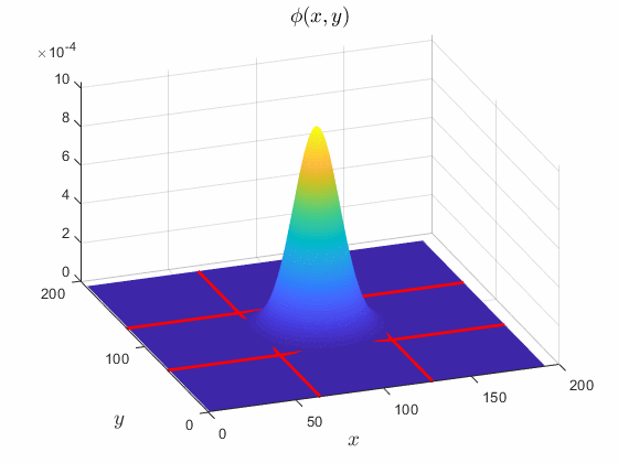
scaling filter. For example, by default the waveletScattering2 function creates a wavelet image scattering network
for the image size 128-by-128 and an invariance scale of 64. The following surface
plot shows the scaling function used in the network. The intersecting red lines form
a 64-by-64 square.

Quality Factors and Filter Banks
When creating a wavelet scattering network, in addition to the invariance scale, you also set the quality factors for the scattering filter banks. The quality factor for each filter bank is the number of wavelet filters per octave. The wavelet transform discretizes the scales using the specified number of wavelet filters.
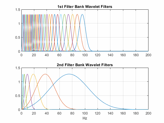
This plot shows the wavelet filters in the network created by waveletScattering. The invariance scale is one second and sampling
frequency is 200 Hz. The first filter bank has the default quality value of 8, and the
second filter bank has the default quality factor of 1.

For image data, large quality factors are not necessary. Large values also result in
significant computational overhead. By default waveletScattering2 creates a network with two filter banks each with a
quality factor of 1. This plot shows the wavelet center frequencies for a wavelet image
scattering network with two filter banks. The first filter bank has a quality factor of
2, and the second filter bank has a quality factor of 1. The number of rotations per
filter bank is 6.

In Practice
With the proper choice of wavelets, the scattering transform is nonexpansive. Energy dissipates as you iterate through the network. As the order m increases, the energy of the mth-order scalogram coefficients and scattering coefficients rapidly converges to 0 [3]. Energy dissipation has a practical benefit. You can limit the number of wavelet filter banks in the network with a minimal loss of signal energy. Published results show that the energy of the third-order scattering coefficients can fall below one percent. For most applications, a network with two wavelet filter banks is sufficient.
Consider the tree view of the wavelet time scattering network. Suppose that there are
M wavelets in the first filter bank, and N
wavelets in the second filter bank. The number of wavelet filters in each filter bank do
not have to be large before a naive implementation becomes unfeasible. Efficient
implementations take advantage of the lowpass nature of the modulus function and
critically downsample the scattering and scalogram coefficients. These strategies were
pioneered by Andén, Mallat, Lostanlen, and Oyallon [4]
[6]
[7] in order to make
scattering transforms computationally practical while maintaining their ability to
produce low-variance data representations for learning. By default, waveletScattering and waveletScattering2 create networks that critically downsample the
coefficients.
References
[1] LeCun, Y., B. Boser, J. S. Denker, D. Henderson, R. E. Howard, W. Hubbard, and L. D. Jackel. "Handwritten Digit Recognition with a Back-Propagation Network." In Advances in Neural Information Processing Systems (NIPS 1989) (D. Touretzky, ed.). 396–404. Denver, CO: Morgan Kaufmann, Vol 2, 1990.
[2] Mallat, Stéphane. “Group Invariant Scattering.” Communications on Pure and Applied Mathematics 65, no. 10 (October 2012): 1331–98. https://doi.org/10.1002/cpa.21413.
[3] Bruna, Joan, and Stéphane Mallat. “Invariant Scattering Convolution Networks.” IEEE Transactions on Pattern Analysis and Machine Intelligence 35, no. 8 (August 2013): 1872–86. https://doi.org/10.1109/TPAMI.2012.230.
[4] Anden, Joakim, and Stéphane Mallat. “Deep Scattering Spectrum.” IEEE Transactions on Signal Processing 62, no. 16 (August 2014): 4114–28. https://doi.org/10.1109/TSP.2014.2326991.
[5] Mallat, Stéphane. “Understanding Deep Convolutional Networks.” Philosophical Transactions of the Royal Society A: Mathematical, Physical and Engineering Sciences 374, no. 2065 (April 13, 2016): 20150203. https://doi.org/10.1098/rsta.2015.0203.
[6] Lostanlen, Vincent. Scattering.m — a MATLAB® toolbox for wavelet scattering. https://github.com/lostanlen/scattering.m.
[7] Oyallon, Edouard. Webpage of Edouard Oyallon. https://edouardoyallon.github.io/.
[8] Sifre, Laurent, and Stéphane Mallat. “Rigid-Motion Scattering for Texture Classification,” 2014. https://doi.org/10.48550/ARXIV.1403.1687.
[9] Sifre, Laurent, and Stéphane Mallat. “Rotation, Scaling and Deformation Invariant Scattering for Texture Discrimination.” In 2013 IEEE Conference on Computer Vision and Pattern Recognition, 1233–40. Portland, OR, USA: IEEE, 2013. https://doi.org/10.1109/CVPR.2013.163.
[10] ScatNet. https://www.di.ens.fr/data/software/scatnet/.
[11] Kymatio. https://www.kymat.io/.
See Also
Objects
Topics
- Wavelet Time Scattering for ECG Signal Classification
- Wavelet Time Scattering Classification of Phonocardiogram Data
- Spoken Digit Recognition with Wavelet Scattering and Deep Learning
- Texture Classification with Wavelet Image Scattering
- Digit Classification with Wavelet Scattering
- Detect Air Compressor Sounds in Simulink Using Wavelet Scattering (DSP System Toolbox)
- Detect Anomalies in ECG Data Using Wavelet Scattering and LSTM Autoencoder in Simulink (DSP System Toolbox)
- Joint Time-Frequency Scattering