Wavelet Time Scattering for ECG Signal Classification

Data Description

This example uses ECG data obtained from three groups, or classes, of people: persons with cardiac arrhythmia, persons with congestive heart failure, and persons with normal sinus rhythms. The example uses 162 ECG recordings from three PhysioNet databases: MIT-BIH Arrhythmia Database [3][5], MIT-BIH Normal Sinus Rhythm Database [3], and The BIDMC Congestive Heart Failure Database [2][3]. In total, there are 96 recordings from persons with arrhythmia, 30 recordings from persons with congestive heart failure, and 36 recordings from persons with normal sinus rhythms. The goal is to train a classifier to distinguish between arrhythmia (ARR), congestive heart failure (CHF), and normal sinus rhythm (NSR).

Download Data

The first step is to download the data from the GitHub repository. To download the data, click Code and select Download ZIP. Save the file physionet_ECG_data-main.zip in a folder where you have write permission. The instructions for this example assume you have downloaded the file to your temporary directory, (tempdir in MATLAB®). Modify the subsequent instructions for unzipping and loading the data if you choose to download the data in a folder different from tempdir.

The file physionet_ECG_data-main.zip contains

and ECGData.zip contains

ECGData.mat holds the data used in this example. The .txt file, Modified_physionet_data.txt, is required by PhysioNet's copying policy and provides the source attributions for the data as well as a description of the pre-processing steps applied to each ECG recording.

Load Files

If you followed the download instructions in the previous section, enter the following commands to unzip the two archive files.

unzip(fullfile(tempdir,"physionet_ECG_data-main.zip"),tempdir)
unzip(fullfile(tempdir,"physionet_ECG_data-main","ECGData.zip"), ...
    fullfile(tempdir,"ECGData"))

After you unzip the ECGData.zip file, load the data into your workspace.

load(fullfile(tempdir,"ECGData","ECGData.mat"))

ECGData is a structure array with two fields: Data and Labels. Data is a 162-by-65536 matrix where each row is an ECG recording sampled at 128 hertz. Each ECG time series has a total duration of 512 seconds. Labels is a 162-by-1 cell array of diagnostic labels, one for each row of Data. The three diagnostic categories are: 'ARR' (arrhythmia), 'CHF' (congestive heart failure), and 'NSR' (normal sinus rhythm).

Create Training and Test Data

Randomly split the data into two sets - training and test data sets. The helper function helperRandomSplit performs the random split. helperRandomSplit accepts the desired split percentage for the training data and ECGData. The helperRandomSplit function outputs two data sets along with a set of labels for each. Each row of trainData and testData is an ECG signal. Each element of trainLabels and testLabels contains the class label for the corresponding row of the data matrices. In this example, we randomly assign 70% percent of the data in each class to the training set. The remaining 30% is held out for testing (prediction) and are assigned to the test set.

percent_train = 70;
[trainData,testData,trainLabels,testLabels] = ...
    helperRandomSplit(percent_train,ECGData);

There are 113 records in the trainData set and 49 records in testData. By design the training data contains 69.75% (113/162) of the data. Recall that the ARR class represents 59.26% of the data (96/162), the CHF class represents 18.52% (30/162), and the NSR class represents 22.22% (36/162). Examine the percentage of each class in the training and test sets. The percentages in each are consistent with the overall class percentages in the data set.

Ctrain = countcats(categorical(trainLabels))./numel(trainLabels).*100

Ctrain = 3×1

   59.2920
   18.5841
   22.1239

Ctest = countcats(categorical(testLabels))./numel(testLabels).*100

Ctest = 3×1

   59.1837
   18.3673
   22.4490

Plot Samples

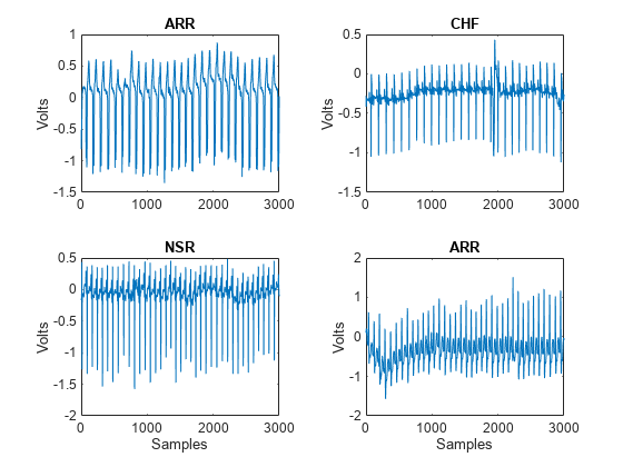
Plot the first few thousand samples of four randomly selected records from ECGData. The helper function helperPlotRandomRecords does this. helperPlotRandomRecords accepts ECGData and a random seed as input. The initial seed is set at 14 so that at least one record from each class is plotted. You can execute helperPlotRandomRecords with ECGData as the only input argument as many times as you wish to get a sense of the variety of ECG waveforms associated with each class. You can find the source code for this and all helper functions in the Supporting Functions section at the end of this example.

helperPlotRandomRecords(ECGData,14)

Wavelet Time Scattering

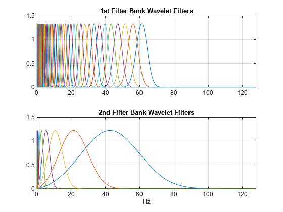
The key parameters to specify in a wavelet time scattering network are the scale of the time invariant, the number of wavelet transforms, and the number of wavelets per octave in each of the wavelet filter banks. In many applications, the cascade of two filter banks is sufficient to achieve good performance. In this example, we construct a wavelet time scattering network with the default filter banks: 8 wavelets per octave in the first filter bank and 1 wavelet per octave in the second filter bank. The invariance scale is set to 150 seconds.

N = size(ECGData.Data,2);
sn = waveletScattering(SignalLength=N,InvarianceScale=150, ...
    SamplingFrequency=128);

You can visualize the wavelet filters in the two filter banks with the following.

[fb,f,filterparams] = filterbank(sn);
figure
tiledlayout(2,1)
nexttile
plot(f,fb{2}.psift)
xlim([0 128])
grid on
title("1st Filter Bank Wavelet Filters")
nexttile
plot(f,fb{3}.psift)
xlim([0 128])
grid on
title("2nd Filter Bank Wavelet Filters")
xlabel("Hz")

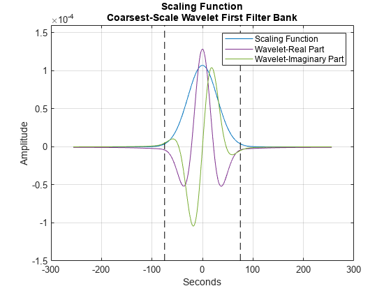
To demonstrate the invariance scale, obtain the inverse Fourier transform of the scaling function and center it at 0 seconds in time. The two vertical black lines mark the -75 and 75 second boundaries. Additionally, plot the real and imaginary parts of the coarsest-scale (lowest frequency) wavelet from the first filter bank. Note that the coarsest-scale wavelet does not exceed the invariant scale determined by the time support of the scaling function. This is an important property of wavelet time scattering.

figure
phi = ifftshift(ifft(fb{1}.phift));
psiL1 = ifftshift(ifft(fb{2}.psift(:,end)));
t = (-2^15:2^15-1).*1/128;
scalplt = plot(t,phi);
hold on
grid on
ylim([-1.5e-4 1.6e-4])
plot([-75 -75],[-1.5e-4 1.6e-4],"k--")
plot([75 75],[-1.5e-4 1.6e-4],"k--")
xlabel("Seconds")
ylabel("Amplitude")
wavplt = plot(t,[real(psiL1) imag(psiL1)]);
legend([scalplt wavplt(1) wavplt(2)], ...
    {"Scaling Function","Wavelet-Real Part","Wavelet-Imaginary Part"})
title({"Scaling Function";"Coarsest-Scale Wavelet First Filter Bank"})
hold off

After constructing the scattering network, obtain the scattering coefficients for the training data as a matrix. When you run featureMatrix with multiple signals, each column is treated as a single signal.

scat_features_train = featureMatrix(sn,trainData');

The output of featureMatrix in this case is 409-by-16-by-113. Each page of the tensor, scat_features_train, is the scattering transform of one signal. The wavelet scattering transform is critically downsampled in time based on the bandwidth of the scaling function. In this case, this results in 16 time windows for each of the 409 scattering paths.

In order to obtain a matrix compatible with the SVM classifier, reshape the multisignal scattering transform into a matrix where each column corresponds to a scattering path and each row is a scattering time window. In this case, you obtain 1808 rows because there are 16 time windows for each of the 113 signals in the training data.

Nwin = size(scat_features_train,2);
scat_features_train = permute(scat_features_train,[2 3 1]);
scat_features_train = reshape(scat_features_train, ...
    size(scat_features_train,1)*size(scat_features_train,2),[]);

Repeat the process for the test data. Initially, scat_features_test is 409-by-16-by-49 because there are 49 ECG waveforms in the training set. After reshaping for the SVM classifier, the feature matrix is 784-by-416.

scat_features_test = featureMatrix(sn,testData');
scat_features_test = permute(scat_features_test,[2 3 1]);
scat_features_test = reshape(scat_features_test, ...
    size(scat_features_test,1)*size(scat_features_test,2),[]);

Because for each signal we obtained 16 scattering windows, we need to create labels to match the number of windows. The helper function createSequenceLabels does this based on the number of windows.

[sequence_labels_train,sequence_labels_test] = createSequenceLabels(Nwin,trainLabels,testLabels);

Cross Validation

For classification, two analyses are performed. The first uses all the scattering data and fits a multi-class SVM with a quadratic kernel. In total there 2592 scattering sequences in the entire dataset, 16 for each of the 162 signals. The error rate, or loss, is estimated using 5-fold cross validation.

scat_features = [scat_features_train; scat_features_test];
allLabels_scat = [sequence_labels_train; sequence_labels_test];
rng(1);
template = templateSVM(...
    KernelFunction="polynomial", ...
    PolynomialOrder=2, ...
    KernelScale="auto", ...
    BoxConstraint=1, ...
    Standardize=true);
classificationSVM = fitcecoc(...
    scat_features, ...
    allLabels_scat, ...
    Learners=template, ...
    Coding="onevsone", ...
    ClassNames={'ARR';'CHF';'NSR'});
kfoldmodel = crossval(classificationSVM,KFold=5);

Compute the loss and the confusion matrix. Display the accuracy.

predLabels = kfoldPredict(kfoldmodel);
loss = kfoldLoss(kfoldmodel)*100;
confmatCV = confusionmat(allLabels_scat,predLabels)

confmatCV = 3×3

        1535           0           1
           1         479           0
           0           0         576

fprintf("Accuracy is %2.2f percent.\n",100-loss);

Accuracy is 99.92 percent.

The accuracy is 99.88%, which is quite good but the actual results are better considering that here each time window is classified separately. There are 16 separate classifications for each signal. Use a simple majority vote to obtain a single class prediction for each scattering representation.

classes = categorical({'ARR','CHF','NSR'});
[ClassVotes,ClassCounts] = helperMajorityVote(predLabels,[trainLabels; testLabels],classes);

Determine the actual cross-validation accuracy based on the mode of the class predictions for each set of scattering time windows. If the mode is not unique for a given set, the helper function helperMajorityVote returns a classification error indicated by 'NoUniqueMode'. This results in an extra column in the confusion matrix, which in this case is all zeros because a unique mode exists for each set of scattering predictions.

CVaccuracy = sum(eq(ClassVotes,categorical([trainLabels; testLabels])))/162*100;
fprintf("True cross-validation accuracy is %2.2f percent.\n",CVaccuracy);

True cross-validation accuracy is 100.00 percent.

MVconfmatCV = confusionmat(categorical([trainLabels; testLabels]),ClassVotes);
MVconfmatCV

MVconfmatCV = 4×4

    96     0     0     0
     0    30     0     0
     0     0    36     0
     0     0     0     0

Scattering has correctly classified all the signals in the cross-validated model. If you examine ClassCounts, you see that the 2 misclassified time windows in confmatCV are attributable to 2 signals where 15 of the 16 scattering windows were classified correctly.

SVM Classification

For the next analysis, we fit a multi-class quadratic SVM to the training data only (70%) and then use that model to make predictions on the 30% of the data held out for testing. There are 49 data records in the test set. Use a majority vote on the individual scattering windows.

model = fitcecoc(...
     scat_features_train, ...
     sequence_labels_train, ...
     Learners=template, ...
     Coding="onevsone", ...
     ClassNames={'ARR','CHF','NSR'});
predLabels = predict(model,scat_features_test);
[TestVotes,TestCounts] = helperMajorityVote(predLabels,testLabels,classes);
testaccuracy = sum(eq(TestVotes,categorical(testLabels)))/numel(testLabels)*100;
fprintf("The test accuracy is %2.2f percent. \n",testaccuracy);

The test accuracy is 97.96 percent. 

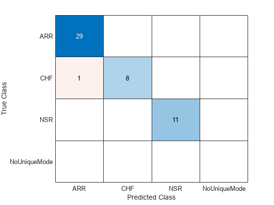
confusionchart(categorical(testLabels),TestVotes)

The classification accuracy on the test dataset is approximately 98%. The confusion matrix shows that one CHF record is misclassified as ARR. All 48 other signals are correctly classified.

Summary

This example used wavelet time scattering and an SVM classifier to classify ECG waveforms into one of three diagnostic classes. Wavelet scattering proved to be a powerful feature extractor, which required only a minimal set of user-specified parameters to yield a set of robust features for classification. Compare this with the example Signal Classification Using Wavelet-Based Features and Support Vector Machines, which required a significant amount of expertise to handcraft features to use in classification. With wavelet time scattering, you are only required to specify the scale of the time invariance, the number of filter banks (or wavelet transforms), and the number of wavelets per octave. The combination of a wavelet scattering transform and an SVM classifier yielded 100% classification on a cross-validated model and 98% correct classification when applying an SVM to the scattering transforms of a hold-out test set.

References

Supporting Functions

helperPlotRandomRecords Plots four ECG signals randomly chosen from ECGData.

function helperPlotRandomRecords(ECGData,randomSeed)
% This function is only intended to support the XpwWaveletMLExample. It may
% change or be removed in a future release.

if nargin==2
    rng(randomSeed)
end

M = size(ECGData.Data,1);
idxsel = randperm(M,4);
tiledlayout(2,2)
for numplot = 1:4
    nexttile
    plot(ECGData.Data(idxsel(numplot),1:3000))
    ylabel('Volts')
    if numplot > 2
        xlabel('Samples')
    end
    title(ECGData.Labels{idxsel(numplot)})
end

end

helperMajorityVote Finds the mode in the predicted class labels for each set of scattering time windows. The function returns both the class label modes and the number of class predictions for each set of scattering time windows. If there is no unique mode, helperMajorityVote returns a class label of "error" to indicate that set of scattering windows is a classification error.

function [ClassVotes,ClassCounts] = helperMajorityVote(predLabels,origLabels,classes)
% This function is in support of ECGWaveletTimeScatteringExample. It may
% change or be removed in a future release.

% Make categorical arrays if the labels are not already categorical
predLabels = categorical(predLabels);
origLabels = categorical(origLabels);
% Expects both predLabels and origLabels to be categorical vectors
Npred = numel(predLabels);
Norig = numel(origLabels);
Nwin = Npred/Norig;
predLabels = reshape(predLabels,Nwin,Norig);
assert(size(predLabels,2) == length(origLabels));
ClassCounts = countcats(predLabels);
[~,idx] = max(ClassCounts);
ClassVotes = classes(idx);
% Check for any ties in the maximum values and ensure they are marked as
% error if the mode occurs more than once
modecnt = modecount(predLabels,string(classes));
ClassVotes(modecnt>1) = categorical({'NoUniqueMode'});
ClassVotes = ClassVotes(:);

%-------------------------------------------------------------------------
function modecnt = modecount(predlabels,classes)
% Ensure there is a unique mode
modecnt = zeros(size(predlabels,2),1);
for nc = 1:size(predlabels,2)
    hc = histcounts(predlabels(:,nc),classes);
    hc = hc-max(hc);
    if sum(hc == 0) > 1
        modecnt(nc) = 1;
    end
end

end

end

References

Anden, J., Mallat, S. 2014. Deep scattering spectrum, IEEE Transactions on Signal Processing, 62, 16, pp. 4114-4128.
Baim DS, Colucci WS, Monrad ES, Smith HS, Wright RF, Lanoue A, Gauthier DF, Ransil BJ, Grossman W, Braunwald E. Survival of patients with severe congestive heart failure treated with oral milrinone. J American College of Cardiology 1986 Mar; 7(3):661-670.
Goldberger AL, Amaral LAN, Glass L, Hausdorff JM, Ivanov PCh, Mark RG, Mietus JE, Moody GB, Peng C-K, Stanley HE. PhysioBank, PhysioToolkit,and PhysioNet: Components of a New Research Resource for Complex Physiologic Signals. Circulation. Vol. 101, No. 23, 13 June 2000, pp. e215-e220.
http://circ.ahajournals.org/content/101/23/e215.fullMallat, S., 2012. Group invariant scattering. Communications in Pure and Applied Mathematics, 65, 10, pp. 1331-1398.
Moody GB, Mark RG. The impact of the MIT-BIH Arrhythmia Database. IEEE Eng in Med and Biol 20(3):45-50 (May-June 2001). (PMID: 11446209)