waveletScattering

Wavelet time scattering

Description

Use the waveletScattering object to create a network for a wavelet time scattering decomposition using the Gabor (analytic Morlet) wavelet. The network uses wavelets and a lowpass scaling function to generate low-variance representations of real-valued time series data. Wavelet time scattering yields representations insensitive to translations in the input signal without sacrificing class discriminability. You can use the representations as inputs to a classifier. You can specify the duration of translation invariance and the number of wavelet filters per octave. The scattering network also supports time × channel × batch (T×C×B) inputs.

Creation

Syntax

sf = waveletScattering

sf = waveletScattering(Name,Value)

Description

sf = waveletScattering creates a wavelet time scattering network with two filter banks. The first filter bank has a quality (Q) factor of eight wavelets per octave. The second filter bank has a Q factor of one wavelet per octave. By default, waveletScattering assumes a signal input length of 1024 samples. The scale invariance length is 512 samples. By default, waveletScattering uses periodic boundary conditions.

example

sf = waveletScattering(Name,Value) creates a network for wavelet scattering, sf, with Properties specified by one or more Name,Value arguments. Properties can be specified in any order as Name1,Value1,...,NameN,ValueN. Enclose each property name in quotes.

Note

After you create a scattering network, you can change the value of the OversamplingFactor property. Depending on the precision of the network and the input signal, the value of the Precision property can also change. All other network property values remain fixed.

example

Properties

expand all

`SignalLength` — Signal length
`1024` (default) | positive integer ≥ 16

Signal length in samples, specified as a positive integer ≥ 16. If the input to the scattering network is a row vector, SignalLength must match the number of columns in the input data. If the input to the scattering network is a column vector, matrix, or 3-D array, SignalLength must match the number of rows in the data.

Data Types: double

`SamplingFrequency` — Sampling frequency
`1` (default) | positive scalar

Sampling frequency in hertz, specified as a positive scalar. If unspecified, frequencies are in cycles/sample and the Nyquist frequency is ½.

Data Types: double

`InvarianceScale` — Scattering transform invariance scale
one-half of `SignalLength` (default) | positive scalar

Scattering transform invariance scale, specified as a positive scalar. InvarianceScale specifies the translation invariance of the scattering transform. If you do not specify SamplingFrequency, InvarianceScale is measured in samples. If you specify SamplingFrequency, InvarianceScale is measured in seconds.

InvarianceScale cannot exceed SignalLength in samples.

Example: sf = waveletScattering('SignalLength',1000,'SamplingFrequency',200,'InvarianceScale',5) has the largest possible invariance scale.

Data Types: double

`QualityFactors` — Scattering filter bank Q factors
`[8 1]` (default) | positive integer | vector of positive integers

Scattering filter bank Q factors, specified as a positive integer or a vector of positive integers. A filter bank Q factor is the number of wavelet filters per octave. Q factors must be less than or equal to 32 and greater than or equal to 1.

If QualityFactors is specified as a vector, the elements of QualityFactors must be strictly decreasing.

Example: sf = waveletScattering('QualityFactors',[8 2 1]) creates a wavelet scattering network with three filter banks.

Data Types: double

`Boundary` — Signal extension method
`'periodic'` (default) | `'reflection'`

Signal extension method to apply at the boundary:

'periodic' — Extend signal periodically to length 2^ceil(log2(N)), where N is the signal length.
'reflection' — Extend signal by reflection to length 2^ceil(log2(2 N)), where N is the signal length.

The signal is extended to match the length of the wavelet filters. The length of the filters are powers of two.

The signal extension method is for internal operations. Results are downsampled back onto the scale of the original signal before being returned.

`Precision` — Numeric precision of wavelet scattering network
`'double'` (default) | `'single'`

Numeric precision of wavelet scattering network:

'double' — Double precision
'single' — Single precision

If you construct a scattering network with double-precision filters and apply the network to single-precision data, the filters are cast internally to single-precision. Subsequent filtering is done with single precision until a new network is created regardless of input data type. For more information, see the example Wavelet Time Scattering Network Precision.

Specifying Precision as 'single' at construction is useful if you want to use the object with single-precision data and reduce the memory footprint of the scattering network.

`OversamplingFactor` — Oversampling factor
`0` (default) | nonnegative integer | `Inf`

Oversampling factor, specified as a nonnegative integer or Inf. The factor specifies how much the scattering coefficients are oversampled with respect to the critically downsampled values. The factor is on a log₂ scale. By default, OversamplingFactor is set to 0, which corresponds to critically downsampling the coefficients. You can use numCoefficients to determine the number of coefficients obtained for a scattering network. To obtain a fully undecimated scattering transform, set OversamplingFactor to Inf.

Setting OversamplingFactor to a value that would result in more coefficients than samples is equivalent to setting OversamplingFactor to Inf. Increasing the OversamplingFactor significantly increases the computational complexity and memory requirements of the scattering transform.

Example: If sf = waveletScattering('OversamplingFactor',2), the scattering transform returns 2² times as many coefficients for each scattering path with respect to the critically sampled number.

`OptimizePath` — Optimize scattering transform logical
`false` or `0` (default) | `true` or `1`

Optimize scattering transform logical which determines whether the scattering transform reduces the number of scattering paths to compute based on a bandwidth consideration, specified as a numeric or logical 1 (true) or 0 (false).

If you specify OptimizePath as true, the scattering transform excludes scattering paths of order 2 and greater which do not satisfy the following criterion: The center frequency minus ½ the 3-dB bandwidth of the wavelet filter in the (i+1)th filter bank must overlap 0 (DC) plus ½ the 3-dB bandwidth of the wavelet filter in the ith filter bank. If this criterion is not satisfied, the higher-order path is excluded. Setting OptimizePath to true can significantly reduce the number of scattering paths and computational complexity of the scattering transform for most networks.

You can use the paths object function to determine which and how many scattering paths are computed.

Object Functions

`scatteringTransform`	Wavelet 1-D scattering transform
`featureMatrix`	Scattering feature matrix
`log`	Natural logarithm of scattering transform
`filterbank`	Wavelet time scattering filter banks
`littlewoodPaleySum`	Littlewood-Paley sum for wavelet time scattering network
`scattergram`	Visualize 1-D scattering or scalogram coefficients
`centerFrequencies`	Wavelet scattering bandpass center frequencies
`numorders`	Number of orders in wavelet time scattering network
`numfilterbanks`	Number of filter banks in wavelet time scattering network
`numCoefficients`	Number of wavelet scattering coefficients
`paths`	Scattering network paths
`gather`	Collect scattering network properties into local workspace

Examples

collapse all

Wavelet Time Scattering with Default Values

Open Live Script

Create a wavelet time scattering network with default values.

sf = waveletScattering

sf = 
  waveletScattering with properties:

          SignalLength: 1024
       InvarianceScale: 512
        QualityFactors: [8 1]
              Boundary: 'periodic'
     SamplingFrequency: 1
             Precision: 'double'
    OversamplingFactor: 0
          OptimizePath: 0

Plot the wavelet filters used in the first and second filter banks.

[filters,f] = filterbank(sf);
plot(f,filters{2}.psift)
title('First Filter Bank')
xlabel('Cycles/Sample')
ylabel('Magnitude')
grid on

Figure contains an axes object. The axes object with title First Filter Bank, xlabel Cycles/Sample, ylabel Magnitude contains 41 objects of type line.

figure
plot(f,filters{3}.psift)
title('Second Filter Bank')
xlabel('Cycles/Sample')
ylabel('Magnitude')
grid on

Figure contains an axes object. The axes object with title Second Filter Bank, xlabel Cycles/Sample, ylabel Magnitude contains 7 objects of type line.

Plot the Littlewood-Paley sums of the filter banks.

[lpsum,f] = littlewoodPaleySum(sf);
figure
plot(f,lpsum)
legend('1st Filter Bank','2nd Filter Bank')
xlabel('Cycles/Sample')
grid on

Figure contains an axes object. The axes object with xlabel Cycles/Sample contains 2 objects of type line. These objects represent 1st Filter Bank, 2nd Filter Bank.

Apply Wavelet Time Scattering Network

Open Live Script

This example shows how to create and apply a wavelet time scattering network with three filter banks to data.

Load in a data set. Create a scattering network with three filter banks that can be applied to the data.

load handel
disp(['Data Sampling Frequency: ',num2str(Fs),' Hz'])

Data Sampling Frequency: 8192 Hz

sf = waveletScattering('SignalLength',numel(y),...
    'SamplingFrequency',Fs,...
    'QualityFactors',[4 2 1])

sf = 
  waveletScattering with properties:

          SignalLength: 73113
       InvarianceScale: 4.4625
        QualityFactors: [4 2 1]
              Boundary: 'periodic'
     SamplingFrequency: 8192
             Precision: 'double'
    OversamplingFactor: 0
          OptimizePath: 0

Inspect the network. Plot the wavelet filters used in the third filter bank.

[filters,f] = filterbank(sf);
plot(f,filters{4}.psift)
title('Third Filter Bank')
xlabel('Hertz')
ylabel('Magnitude')
grid on

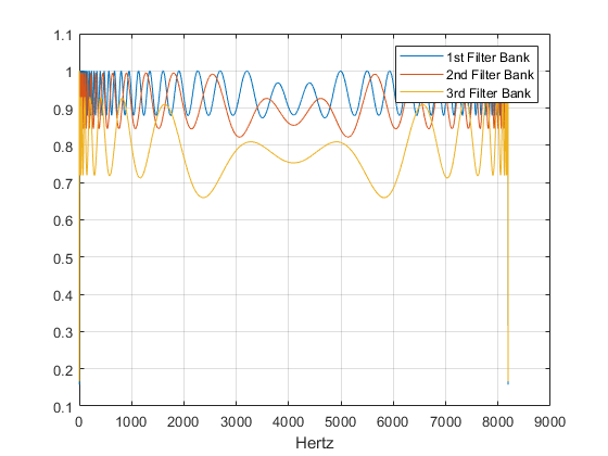
Plot the Littlewood-Paley sums of the three filter banks.

[lpsum,f] = littlewoodPaleySum(sf);
figure
plot(f,lpsum)
xlabel('Hertz')
grid on
legend('1st Filter Bank','2nd Filter Bank','3rd Filter Bank')

Calculate the wavelet 1-D scattering transform of the data for sf. Visualize the scattergram of the scalogram coefficients for the first filter bank.

[S,U] = scatteringTransform(sf,y);
figure
scattergram(sf,U,'FilterBank',1)

Wavelet Time Scattering Network Precision

Open Live Script

This example shows how single-precision input changes the default numeric precision of a wavelet scattering network.

Create a wavelet time scattering network with default values. The precision of the network is double.

sf = waveletScattering

sf = 
  waveletScattering with properties:

          SignalLength: 1024
       InvarianceScale: 512
        QualityFactors: [8 1]
              Boundary: 'periodic'
     SamplingFrequency: 1
             Precision: 'double'
    OversamplingFactor: 0
          OptimizePath: 0

Use the filterbank object function to obtain the scattering filter banks. The filterbank function returns the filter banks in a cell array. Confirm the filters are double precision.

sfFilters = filterbank(sf);
precType = "double";
fprintf("Checking precision: %s\n",precType)

Checking precision: double

fprintf("sfFilters{1}.phift: %d\n", ...
    isa(sfFilters{1}.phift,precType))

sfFilters{1}.phift: 1

for k=2:numel(sfFilters)
    fprintf("sfFilters{%d}.phift: %d\n", ...
        k,isa(sfFilters{k}.phift,precType))
    fprintf("sfFilters{%d}.psift: %d\n", ...
        k,isa(sfFilters{k}.psift,precType))
end

sfFilters{2}.phift: 1

sfFilters{2}.psift: 1

sfFilters{3}.phift: 1

sfFilters{3}.psift: 1

Load the noisy Doppler signal. The signal is double precision.

load noisdopp
isa(noisdopp,"double")

ans = logical
   1

Use the featureMatrix object function to obtain the scattering coefficient matrix for the scattering network and the signal. Confirm the precision of the matrix is double.

smat = featureMatrix(sf,noisdopp);
isa(smat,"double")

ans = logical
   1

Convert the signal to single precision. Obtain the scattering coefficient matrix of the single-precision signal using the scattering network. Confirm the matrix precision is single.

noisdoppSingle = single(noisdopp);
smatSingle = featureMatrix(sf,noisdoppSingle);
isa(smatSingle,"single")

ans = logical
   1

Confirm that by using single-precision input, the numeric precision of the scattering network has changed to single.

sf

sf = 
  waveletScattering with properties:

          SignalLength: 1024
       InvarianceScale: 512
        QualityFactors: [8 1]
              Boundary: 'periodic'
     SamplingFrequency: 1
             Precision: 'single'
    OversamplingFactor: 0
          OptimizePath: 0

Use the featureMatrix function to obtain the scattering coefficient matrix for the scattering network and the double-precision signal. Because the numeric precision of the network is now single, the matrix precision is single.

smatSingle2 = featureMatrix(sf,noisdopp);
isa(smatSingle2,"single")

ans = logical
   1

Use the filterbank function to obtain the filter banks. Confirm the filters have changed to single precision.

sfFiltersSingle = filterbank(sf);
precType = "single";
fprintf("Checking precision: %s\n",precType)

Checking precision: single

fprintf("sfFiltersSingle{1}.phift: %d\n", ...
    isa(sfFiltersSingle{1}.phift,precType))

sfFiltersSingle{1}.phift: 1

for k=2:numel(sfFilters)
    fprintf("sfFiltersSingle{%d}.phift: %d\n", ...
        k,isa(sfFiltersSingle{k}.phift,precType))
    fprintf("sfFiltersSingle{%d}.psift: %d\n", ...
        k,isa(sfFiltersSingle{k}.psift,precType))
end

sfFiltersSingle{2}.phift: 1

sfFiltersSingle{2}.psift: 1

sfFiltersSingle{3}.phift: 1

sfFiltersSingle{3}.psift: 1

More About

expand all

Time Windows

You set the invariance scale based on how much insensitivity to time-shifts in the data you want. Equivalently, the invariance scale is the length of the Gaussian smoothing function the scattering transform convolves with the scalogram coefficients. The longer the Gaussian is in time (samples), the narrower the support (bandwidth) of its Fourier transform. You can downsample the output of the smoothing operation. In the context of wavelet scattering, the term "time windows" refers to the number of samples obtained after downsampling the output of the smoothing operation.

When you use the default waveletScattering network, the scattering transform downsamples the output of the smoothing operation as much as possible without causing aliasing. If you want to downsample less than the maximum amount, set the oversampling factor of the network to a nonzero value. That, in turn, affects the number of time windows, because you will keep more samples from the output of the application of the Gaussian smoothing filter to the scalograms. By changing the oversampling factor, you can obtain more time windows for the same given invariance scale.

References

[1] Andén, Joakim, and Stéphane Mallat. “Deep Scattering Spectrum.” IEEE Transactions on Signal Processing 62, no. 16 (August 2014): 4114–28. https://doi.org/10.1109/TSP.2014.2326991.

[2] Mallat, Stéphane. “Group Invariant Scattering.” Communications on Pure and Applied Mathematics 65, no. 10 (October 2012): 1331–98. https://doi.org/10.1002/cpa.21413.

Extended Capabilities

C/C++ Code Generation
Generate C and C++ code using MATLAB® Coder™.

Usage notes and limitations:

If specified, 'Precision' and 'Boundary' values must be coder.Constant.
QualityFactors cannot be variable sized.
waveletScattering is a handle class, so you must use an entry-point function.
To generate optimized code that uses SIMD intrinsics and runs on ARM^® Cortex^®-A 32-bit/64-bit processors, you must install the Embedded Coder^® Support Package for AMD SoC Devices. The support package for Xilinx^® Zynq^® Platform ships the ARM cross-compiler toolchains and enables deployment on ARM Cortex-A processors. The MATLAB^® Support Package for Raspberry Pi^® Hardware enables a direct deployment of optimized code on ARM devices. For an example, see Generate and Deploy Optimized Code for Wavelet Time Scattering on ARM Targets. (since R2023a)

GPU Arrays
Accelerate code by running on a graphics processing unit (GPU) using Parallel Computing Toolbox™.

The waveletScattering function fully supports GPU arrays. To run the function on a GPU, specify the input data as a gpuArray (Parallel Computing Toolbox). For more information, see Run MATLAB Functions on a GPU (Parallel Computing Toolbox).

Version History

Introduced in R2018b

expand all

R2023a: Use object function `gather` to collect properties into local workspace

You can use the object function gather to collect all the properties of a waveletScattering object from the GPU device into your workspace. This support requires Parallel Computing Toolbox™.

R2023a: Generate optimized C++ code for ARM Cortex-A 32-bit/64-bit processors

You can generate optimized C++ code that uses SIMD intrinsics and runs on ARM Cortex-A 32-bit/64-bit processors. For more information, see Code Generation.

R2021a: `waveletScattering` property `Decimate` has been removed

The waveletScattering property Decimate has been removed. Use the property OversamplingFactor instead.

Functionality	What Happens When You Use This Functionality?	Use This Instead	Compatibility Considerations
`Decimate` property	Errors	`OversamplingFactor`	Replace all instances of `'Decimate',true` with `'OversamplingFactor',0`. Replace all instances of `'Decimate',false` with `'OversamplingFactor',Inf`.

R2021a: Highest wavelet center frequency is computed using geometric mean

Starting in R2021a, the highest wavelet center frequency is computed using the geometric mean. The method for determining how to space linearly those frequencies lower than the invariance scale has also changed. These changes improve the Littlewood-Paley sums of the resulting filter banks.

Center frequencies are logarithmically spaced from the highest frequency to the frequency that corresponds to the invariance scale. Starting in R2021a, depending on scattering network parameters such as the invariance scale, the number of filters you obtain may be different than in previous releases. The method for applying the filters to compute the scattering and scalogram coefficients has not changed.

waveletScattering

Description

Creation

Syntax

Description

Properties

`SignalLength` — Signal length
`1024` (default) | positive integer ≥ 16

`SamplingFrequency` — Sampling frequency
`1` (default) | positive scalar

`InvarianceScale` — Scattering transform invariance scale
one-half of `SignalLength` (default) | positive scalar

`QualityFactors` — Scattering filter bank Q factors
`[8 1]` (default) | positive integer | vector of positive integers

`Boundary` — Signal extension method
`'periodic'` (default) | `'reflection'`

`Precision` — Numeric precision of wavelet scattering network
`'double'` (default) | `'single'`

`OversamplingFactor` — Oversampling factor
`0` (default) | nonnegative integer | `Inf`

`OptimizePath` — Optimize scattering transform logical
`false` or `0` (default) | `true` or `1`

Object Functions

Examples

Wavelet Time Scattering with Default Values

Apply Wavelet Time Scattering Network

Wavelet Time Scattering Network Precision

More About

Time Windows

References

Extended Capabilities

C/C++ Code Generation
Generate C and C++ code using MATLAB® Coder™.

GPU Arrays
Accelerate code by running on a graphics processing unit (GPU) using Parallel Computing Toolbox™.

Version History

R2023a: Use object function `gather` to collect properties into local workspace

R2023a: Generate optimized C++ code for ARM Cortex-A 32-bit/64-bit processors

R2021a: `waveletScattering` property `Decimate` has been removed

R2021a: Highest wavelet center frequency is computed using geometric mean

See Also

Functions

Objects

Blocks

Topics

waveletScattering

Description

Creation

Syntax

Description

Properties

SignalLength — Signal length 1024 (default) | positive integer ≥ 16

SamplingFrequency — Sampling frequency 1 (default) | positive scalar

InvarianceScale — Scattering transform invariance scale one-half of SignalLength (default) | positive scalar

QualityFactors — Scattering filter bank Q factors [8 1] (default) | positive integer | vector of positive integers

Boundary — Signal extension method 'periodic' (default) | 'reflection'

Precision — Numeric precision of wavelet scattering network 'double' (default) | 'single'

OversamplingFactor — Oversampling factor 0 (default) | nonnegative integer | Inf

OptimizePath — Optimize scattering transform logical false or 0 (default) | true or 1

Object Functions

Examples

Wavelet Time Scattering with Default Values

Apply Wavelet Time Scattering Network

Wavelet Time Scattering Network Precision

More About

Time Windows

References

Extended Capabilities

C/C++ Code Generation Generate C and C++ code using MATLAB® Coder™.

GPU Arrays Accelerate code by running on a graphics processing unit (GPU) using Parallel Computing Toolbox™.

Version History

R2023a: Use object function gather to collect properties into local workspace

R2023a: Generate optimized C++ code for ARM Cortex-A 32-bit/64-bit processors

R2021a: waveletScattering property Decimate has been removed

R2021a: Highest wavelet center frequency is computed using geometric mean

See Also

Functions

Objects

Blocks

Topics

`SignalLength` — Signal length
`1024` (default) | positive integer ≥ 16

`SamplingFrequency` — Sampling frequency
`1` (default) | positive scalar

`InvarianceScale` — Scattering transform invariance scale
one-half of `SignalLength` (default) | positive scalar

`QualityFactors` — Scattering filter bank Q factors
`[8 1]` (default) | positive integer | vector of positive integers

`Boundary` — Signal extension method
`'periodic'` (default) | `'reflection'`

`Precision` — Numeric precision of wavelet scattering network
`'double'` (default) | `'single'`

`OversamplingFactor` — Oversampling factor
`0` (default) | nonnegative integer | `Inf`

`OptimizePath` — Optimize scattering transform logical
`false` or `0` (default) | `true` or `1`

C/C++ Code Generation
Generate C and C++ code using MATLAB® Coder™.

GPU Arrays
Accelerate code by running on a graphics processing unit (GPU) using Parallel Computing Toolbox™.

R2023a: Use object function `gather` to collect properties into local workspace

R2021a: `waveletScattering` property `Decimate` has been removed