cwtfilterbank
Continuous wavelet transform filter bank
Description
Use cwtfilterbank to create a continuous wavelet
transform (CWT) filter bank. The default wavelet used in the filter bank is the analytic
Morse (3,60) wavelet. You can vary the time-bandwidth and symmetry parameters for the
Morse wavelets, to tune the Morse wavelet for your needs. You can also use the analytic
Morlet (Gabor) wavelet or bump wavelet. When analyzing multiple signals in
time-frequency, for improved computational efficiency, you can precompute the filters
once and then pass the filter bank as input to cwt. With the filter bank, you can visualize wavelets in time and
frequency. You can also create filter banks with specific frequency or period ranges,
and measure 3-dB bandwidths. You can determine the quality factor for the wavelets in
the filter bank.
Creation
Description
fb = cwtfilterbankfb. The
filters are normalized so that the peak magnitudes for all passbands are
approximately equal to 2. The default filter bank is designed for a signal
with 1024 samples. The default filter bank uses the analytic Morse (3,60)
wavelet. The filter bank uses the default scales: approximately 10 wavelet
bandpass filters per octave (10 voices per octave). The highest-frequency
passband is designed so that the magnitude falls to half the peak value at
the Nyquist frequency.
As implemented, the CWT uses L1 normalization. With L1 normalization, equal amplitude oscillatory components at different scales have equal magnitude in the CWT. L1 normalization provides a more accurate representation of the signal. The amplitudes of the oscillatory components agree with the amplitudes of the corresponding wavelet coefficients. See Sinusoid and Wavelet Coefficient Amplitudes.
fb can be used as input for cwt.
fb = cwtfilterbank(PropertyName=Value)fb with properties using one
or more name-value arguments. Properties can be specified in any order as
Name1=Value1,...,NameN=ValueN.
Note
You cannot change a property value of an existing filter bank. For
example, if you have a filter bank fb with a
SignalLength of 2000, you must create a
second filter bank fb2 to process a signal with
2001 samples. You cannot assign a different
SignalLength to fb.
Properties
Object Functions
wt | Continuous wavelet transform with filter bank |
freqz | CWT filter bank frequency responses |
timeSpectrum | Time-averaged wavelet spectrum |
scaleSpectrum | Scale-averaged wavelet spectrum |
wavelets | CWT filter bank time-domain wavelets |
scales | CWT filter bank scales |
waveletsupport | CWT filter bank time supports |
qfactor | CWT filter bank quality factor |
powerbw | CWT filter bank 3 dB bandwidths |
centerFrequencies | CWT filter bank bandpass center frequencies |
centerPeriods | CWT filter bank bandpass center periods |
Examples
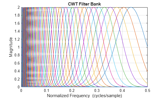
Create a continuous wavelet transform filter bank.
fb = cwtfilterbank
fb =
  cwtfilterbank with properties:

      VoicesPerOctave: 10
              Wavelet: "Morse"
    SamplingFrequency: 1
       SamplingPeriod: []
         PeriodLimits: []
         SignalLength: 1024
      FrequencyLimits: []
        TimeBandwidth: 60
    WaveletParameters: []
             Boundary: "reflection"
Plot the magnitude frequency response.
freqz(fb)
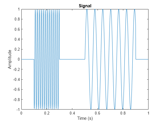
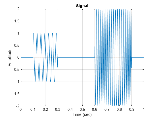
Create two sine waves with frequencies of 16 and 64 Hz. The data is sampled at 1000 Hz. Plot the signal.
Fs = 1e3;
t = 0:1/Fs:1-1/Fs;
x = cos(2*pi*64*t).*(t>=0.1 & t<0.3)+ ...
    sin(2*pi*16*t).*(t>=0.5 & t<0.9);
plot(t,x)
title("Signal")
xlabel("Time (s)")
ylabel("Amplitude")
Create a CWT filter bank for the signal. Plot the frequency responses of the wavelets in the filter bank.
fb = cwtfilterbank(SignalLength=numel(t),SamplingFrequency=Fs);
figure
freqz(fb)
title("Frequency Responses — Morse (3,60) Wavelet")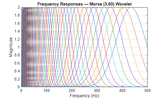
The analytic Morse (3,60) wavelet is the default wavelet in the filter bank. The wavelet has a time-bandwidth product equal to 60. Create a second filter bank identical to the first filter bank but instead uses the analytic Morse (3,5) wavelet. Plot the frequency responses of the wavelets in the second filter bank.
fb3x5 = cwtfilterbank(SignalLength=numel(t),SamplingFrequency=Fs,...
    TimeBandwidth=5);
figure
freqz(fb3x5)
title("Frequency Responses — Morse (3,5) Wavelet")
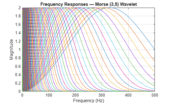
Observe that the frequency responses are wider than in the first filter bank. The Morse (3,60) wavelet is better localized in frequency than the Morse (3,5) wavelet. Apply each filter bank to the signal and plot the resulting scalograms. Observe that the Morse (3,60) wavelet has better frequency resolution than the Morse (3,5) wavelet.
figure
cwt(x,FilterBank=fb)
title("Magnitude Scalogram — Morse (3,60)")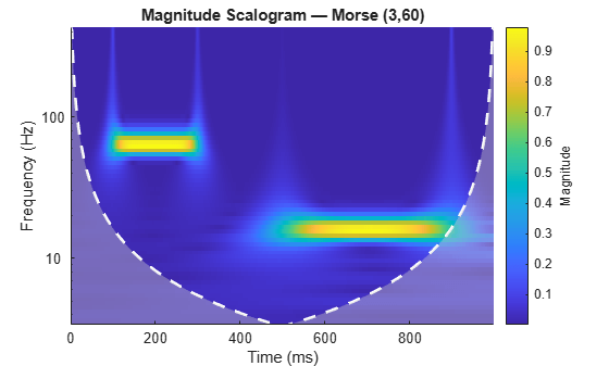
figure
cwt(x,FilterBank=fb3x5)
title("Magnitude Scalogram — Morse (3,5)")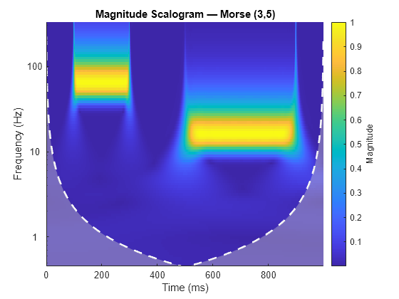
This example shows that the amplitudes of oscillatory components in a signal agree with the amplitudes of the corresponding wavelet coefficients.
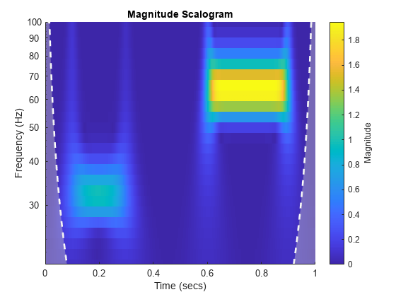
Create a signal composed of two sinusoids with disjoint support in time. One sinusoid has a frequency of 32 Hz and amplitude equal to 1. The other sinusoid has a frequency of 64 Hz and amplitude equal to 2. The signal is sampled for one second at 1000 Hz. Plot the signal.
frq1 = 32;
amp1 = 1;
frq2 = 64;
amp2 = 2;

Fs = 1e3;
t = 0:1/Fs:1;
x = amp1*sin(2*pi*frq1*t).*(t>=0.1 & t<0.3)+...
    amp2*sin(2*pi*frq2*t).*(t>0.6 & t<0.9);

plot(t,x)
grid on
xlabel("Time (sec)")
ylabel("Amplitude")
title("Signal")
Create a CWT filter bank that can be applied to the signal. Since the signal component frequencies are known, set the frequency limits of the filter bank to a narrow range that includes the known frequencies. To confirm the range, plot the magnitude frequency responses for the filter bank.
fb = cwtfilterbank(SignalLength=numel(x),SamplingFrequency=Fs,...
    FrequencyLimits=[20 100]);
freqz(fb)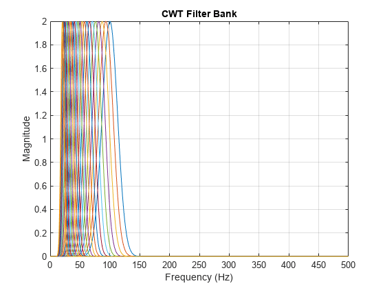
Use cwt and the filter bank to plot the scalogram of the signal.
cwt(x,FilterBank=fb)
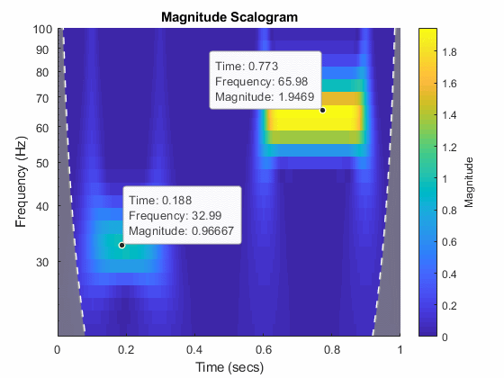
Use a data cursor to confirm that the amplitudes of the wavelet coefficients are essentially equal to the amplitudes of the sinusoidal components.
This example shows how to vary the time-bandwidth parameter of the generalized Morse wavelet to approximate the analytic Morlet wavelet.
Generalized Morse wavelets are a family of exactly analytic wavelets. Morse wavelets have two parameters, symmetry and time-bandwidth product. You can vary these parameters to obtain analytic wavelets with different properties and behaviors. For additional information, see Morse Wavelets and the references therein.
Load the seismograph data recorded during the 1995 Kobe earthquake. The data are seismograph (vertical acceleration, nm/sq.sec) measurements recorded at Tasmania University, Hobart, Australia on 16 January 1995 beginning at 20:56:51 (GMT) and continuing for 51 minutes at 1 second intervals. Create a CWT filter bank with default settings that can be applied to the data. Use the filter bank to generate the scalogram.
load kobe
fb = cwtfilterbank(SignalLength=numel(kobe), ...
    SamplingFrequency=1);
cwt(kobe,FilterBank=fb)
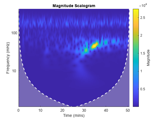
The magnitude of the wavelet coefficients is large in the frequency range from 10 mHz to 100 mHz. Create a new filter bank with frequency limits set to these values. Generate the scalogram.
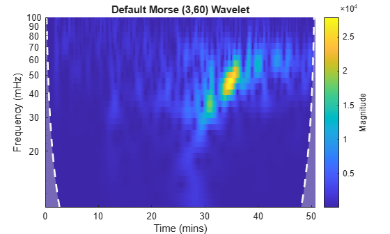
fb2 = cwtfilterbank(SignalLength=numel(kobe), ...
    SamplingFrequency=1, ...
    FrequencyLimits=[1e-2 1e-1]);
cwt(kobe,FilterBank=fb2)
title("Default Morse (3,60) Wavelet")
By default, cwtfilterbank uses the Morse (3,60) wavelet. Create a filter bank using the analytic Morlet wavelet with the same frequency limits. Generate a scalogram and compare with the scalogram generated by the Morse (3,60) wavelet.
fbMorlet = cwtfilterbank(SignalLength=numel(kobe), ...
    SamplingFrequency=1, ...
    FrequencyLimits=[1e-2 1e-1], ...
    Wavelet="amor");
cwt(kobe,FilterBank=fbMorlet)
title("Analytic Morlet Wavelet")
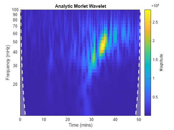
The Morlet wavelet is not as well localized in frequency as the (3,60) Morse wavelet. However, by varying the time-bandwidth product, you can create a Morse wavelet with properties similar to the Morlet wavelet.
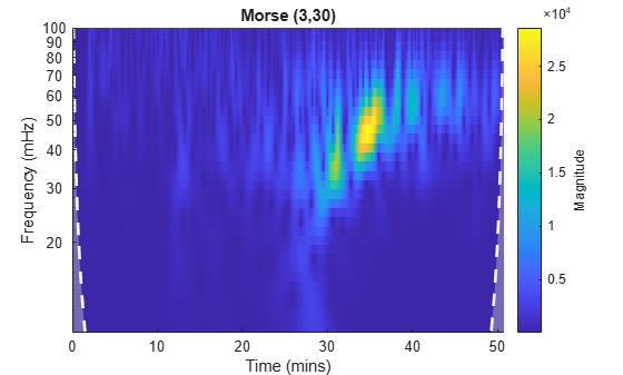
Create a filter bank using the Morse wavelet with a time-bandwidth value of 30 [2], with frequency limits as above. Generate the scalogram of the seismograph data. Note there is smearing in frequency nearly identical to the Morlet results.
fbMorse = cwtfilterbank(SignalLength=numel(kobe), ...
    SamplingFrequency=1, ...
    FrequencyLimits=[1e-2 1e-1], ...
    TimeBandwidth=30);
cwt(kobe,FilterBank=fbMorse)
title("Morse (3,30)")
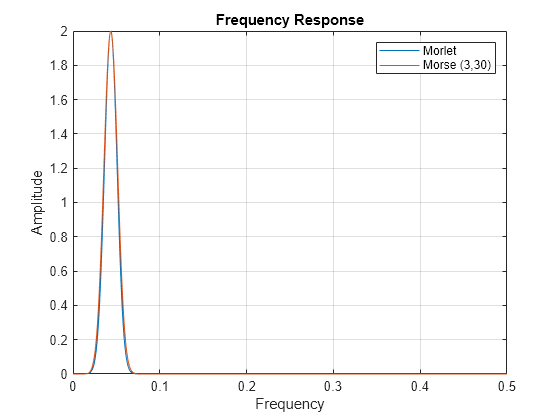
Now examine the wavelets associated with the fbMorlet and fbMorse filter banks. From both filter banks, obtain the wavelet center frequencies, filter frequency responses, and time-domain wavelets. Confirm the center frequencies are nearly identical.
cfMorlet = centerFrequencies(fbMorlet);
[frMorlet,fMorlet] = freqz(fbMorlet);
[wvMorlet,tMorlet] = wavelets(fbMorlet);
cfMorse = centerFrequencies(fbMorse);
[frMorse,fMorse] = freqz(fbMorse);
[wvMorse,tMorse] = wavelets(fbMorse);

disp("Number of Center Frequencies: "+num2str(length(cfMorlet)));
Number of Center Frequencies: 34
disp("Maximum difference: "+num2str(max(abs(cfMorlet-cfMorse))));Maximum difference: 1.3878e-17
Each filter bank contains the same number of wavelets. Choose a center frequency, and plot the frequency response of the associated filter from each filter bank. Confirm the responses are nearly identical.
wv = 13;
figure
plot(fMorlet,frMorlet(wv,:));
hold on
plot(fMorse,frMorse(wv,:));
grid on
hold off
title("Frequency Response")
xlabel("Frequency")
ylabel("Amplitude")
legend("Morlet","Morse (3,30)")
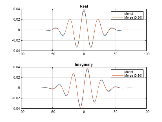
Plot the time-domain wavelets associated with the same center frequency. Confirm they are nearly identical.
figure
subplot(2,1,1)
plot(tMorlet,real(wvMorlet(wv,:)))
hold on
plot(tMorse,real(wvMorse(wv,:)))
grid on
hold off
title("Real")
legend("Morlet","Morse (3,30)")
xlim([-100 100])
subplot(2,1,2)
plot(tMorlet,imag(wvMorlet(wv,:)))
hold on
plot(tMorse,imag(wvMorse(wv,:)))
grid on
hold off
title("Imaginary")
legend("Morlet","Morse (3,30)")
xlim([-100 100])
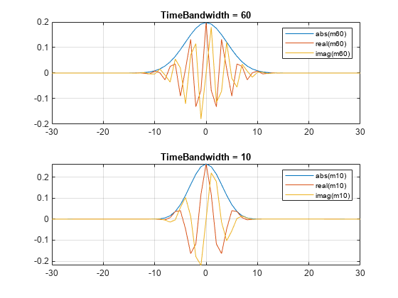
This example shows that increasing the time-bandwidth product of the Morse wavelet creates a wavelet with more oscillations under its envelope. Increasing narrows the wavelet in frequency.
Create two filter banks. One filter bank has the default TimeBandwidth value of 60. The second filter bank has a TimeBandwidth value of 10. The SignalLength for both filter banks is 4096 samples.
sigLen = 4096;
fb60 = cwtfilterbank(SignalLength=sigLen);
fb10 = cwtfilterbank(SignalLength=sigLen,TimeBandwidth=10);
Obtain the time-domain wavelets for the filter banks.
[psi60,t] = wavelets(fb60);
[psi10,~] = wavelets(fb10);
Use the scales function to find the mother wavelet for each filter bank.
sca60 = scales(fb60);
sca10 = scales(fb10);
[~,idx60] = min(abs(sca60-1));
[~,idx10] = min(abs(sca10-1));
m60 = psi60(idx60,:);
m10 = psi10(idx10,:);
Since the time-bandwidth product is larger for the fb60 filter bank, verify the m60 wavelet has more oscillations under its envelope than the m10 wavelet.
tiledlayout(2,1)
nexttile
plot(t,abs(m60))
grid on
hold on
plot(t,real(m60))
plot(t,imag(m60))
hold off
xlim([-30 30])
legend("abs(m60)","real(m60)","imag(m60)")
title("TimeBandwidth = 60")
nexttile
plot(t,abs(m10))
grid on
hold on
plot(t,real(m10))
plot(t,imag(m10))
hold off
xlim([-30 30])
legend("abs(m10)","real(m10)","imag(m10)")
title("TimeBandwidth = 10")
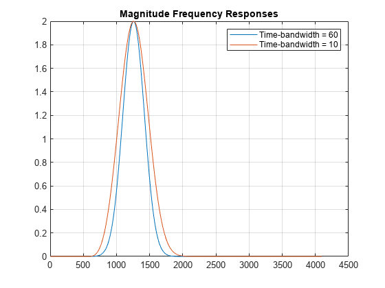
Align the peaks of the m60 and m10 magnitude frequency responses. Verify the frequency response of the m60 wavelet is narrower than the frequency response for the m10 wavelet.
cf60 = centerFrequencies(fb60);
cf10 = centerFrequencies(fb10);

m60cFreq = cf60(idx60);
m10cFreq = cf10(idx10);

freqShift = 2*pi*(m60cFreq-m10cFreq);
x10 = m10.*exp(1j*freqShift*(-sigLen/2:sigLen/2-1));

figure
plot([abs(fft(m60)).' abs(fft(x10)).'])
grid on
legend("Time-Bandwidth = 60","Time-Bandwidth = 10")
title("Magnitude Frequency Responses")
This example shows how using a CWT filter bank can improve computational efficiency when taking the CWT of multiple time series.
Create a 100-by-1024 matrix x. Create a CWT filter bank appropriate for signals with 1024 samples.
x = randn(100,1024);
fb = cwtfilterbank;
Use cwt with default settings to obtain the CWT of a signal with 1024 samples. Create a 3-D array that can contain the CWT coefficients of 100 signals, each of which has 1024 samples.
cfs = cwt(x(1,:));
res = zeros(100,size(cfs,1),size(cfs,2));
Use the cwt function and take the CWT of each row of the matrix x. Display the elapsed time.
tic
for k=1:100
    res(k,:,:) = cwt(x(k,:));
end
toc
Elapsed time is 0.928160 seconds.
Now use the wt object function of the filter bank to take the CWT of each row of x. Display the elapsed time.
tic
for k=1:100
    res(k,:,:) = wt(fb,x(k,:));
end
toc
Elapsed time is 0.393524 seconds.
This example shows how to plot the CWT scalogram in a figure subplot.
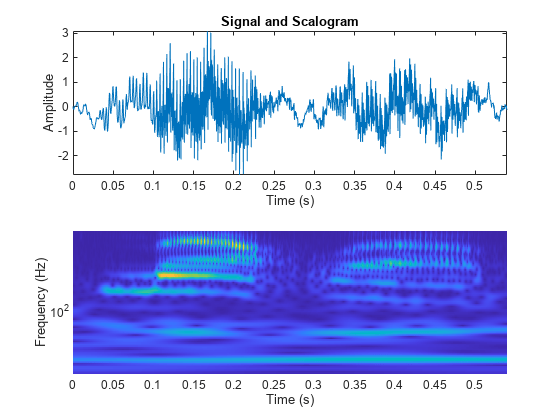
Load the speech sample. The data is sampled at 7418 Hz. Plot the default CWT scalogram.
load mtlb
cwt(mtlb,Fs)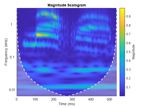
Obtain the CWT of the signal, and the scale-to-frequency conversions of the CWT.
[cfs,frq] = cwt(mtlb,Fs);
The cwt function sets the time and frequency axes in the scalogram. Create a vector representing the sample times.
tms = (0:numel(mtlb)-1)/Fs;
In a new figure, plot the original signal in the upper subplot and the scalogram in the lower subplot. Plot the frequencies on a logarithmic scale.
figure
tiledlayout(2,1)
nexttile
plot(tms,mtlb)
axis tight
title("Signal and Scalogram")
xlabel("Time (s)")
ylabel("Amplitude")
nexttile
surface(tms,frq,abs(cfs))
axis tight
shading flat
xlabel("Time (s)")
ylabel("Frequency (Hz)")
set(gca,"yscale","log")
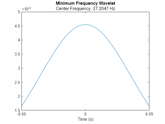
Create a CWT filter bank using the analytic Morlet wavelet. Specify a signal length of 500 samples, a sampling frequency of 5000 Hz, and frequency limits of [20 1000] Hz.
fb = cwtfilterbank(Wavelet="amor",SignalLength=500, ...
    SamplingFrequency=5000, ...
    FrequencyLimits=[20 1000]);
Obtain the lowest and highest bandpass center frequencies from the filter bank. To ensure there is sufficient decay at the beginning and the end of the signal for the largest wavelet in time, the filter bank truncates the minimum desired frequency to the smallest permissible value. The minimum frequency wavelet is such that given the requested wavelet, two standard deviations (in time) of the wavelet occur within the requested signal length.
cf = centerFrequencies(fb);
minfreqFB = min(cf)
minfreqFB =
27.2047
maxfreqFB = max(cf)
maxfreqFB =
1.0000e+03
Plot in the time domain the magnitude of the minimum frequency wavelet.
[psi,t] = wavelets(fb);
plot(t,abs(psi(end,:)))
title("Minimum Frequency Wavelet", ...
    "Center Frequency: "+num2str(minfreqFB)+" Hz")
xlabel("Time (s)")
Use the cwtfreqbounds function to determine the minimum permissible frequency for a signal of length 2500 and a sampling frequency of 5000 Hz using the analytic Morlet wavelet. The minimum permissible frequency is less than 20 Hz.
minf = cwtfreqbounds(2500,5000,Wavelet="amor")minf = 5.4019
Create a new filter bank identical to the first, except specify a signal length of 2500. The lowest bandpass center frequency is much closer to the desired value of 20 Hz.
fb2 = cwtfilterbank(Wavelet="amor",SignalLength=2500, ...
    SamplingFrequency=5000, ...
    FrequencyLimits=[20 1000]);
cf2 = centerFrequencies(fb2);
minfreqFB2 = min(cf2)
minfreqFB2 =
20.6173
Plot the minimum frequency wavelet. The wavelet decays well within the signal length.
[psi,t] = wavelets(fb2);
plot(t,abs(psi(end,:)))
title("Minimum Frequency Wavelet", ...
    "Center Frequency: "+num2str(minfreqFB2)+" Hz")
xlabel("Time (s)")

Tips
The first time you use a filter bank to take the CWT of a signal, the wavelet filters are constructed to have the same datatype as the signal. A warning message is generated when you apply the same filter bank to a signal with a different datatype. Changing datatypes comes with the cost of redesigning or changing the precision of the filter bank. For optimal performance, use a consistent datatype.
When performing multiple CWTs, for example inside a for-loop, the recommended workflow is to first create a
cwtfilterbankobject and then use thewtobject function. This workflow minimizes overhead and maximizes performance. See Using CWT Filter Bank on Multiple Time Series.
References
[1] Lilly, J. M., and S. C. Olhede. “Generalized Morse Wavelets as a Superfamily of Analytic Wavelets.” IEEE Transactions on Signal Processing. Vol. 60, No. 11, 2012, pp. 6036–6041.
[2] Lilly, J. M., and S. C. Olhede. “Higher-Order Properties of Analytic Wavelets.” IEEE Transactions on Signal Processing. Vol. 57, No. 1, 2009, pp. 146–160.
[3] Lilly, J. M. jLab: A data analysis package for MATLAB®, version 1.6.2. 2016. http://www.jmlilly.net/jmlsoft.html.
[4] Lilly, J. M. “Element analysis: a wavelet-based method for analysing time-localized events in noisy time series.” Proceedings of the Royal Society A. Volume 473: 20160776, 2017, pp. 1–28. dx.doi.org/10.1098/rspa.2016.0776.