Main Content

icwt

Inverse continuous 1-D wavelet transform

Description

xrec = icwt(cfs) inverts the continuous wavelet transform (CWT) coefficient matrix cfs using Morlet's single integral formula. icwt assumes that you obtained the CWT using cwt with the default analytic Morse (3,60) wavelet. This wavelet has a symmetry of 3 and a time bandwidth of 60. icwt also assumes that the CWT uses default scales.

example

xrec = icwt(cfs,wname) uses the analytic wavelet wname to invert the CWT. The specified wavelet must be the same wavelet used in cwt.

example

xrec = icwt(___,f,freqrange) inverts the CWT over the frequency range specified in freqrange. f is the scale-to-frequency conversion obtained from cwt.

In R2022a: If you invert the CWT over a specified frequency range, you must precede those inputs either by a wavelet name or an empty input for the default Morse wavelet. For more information, see icwt behavior change.

example

xrec = icwt(___,period,periodrange) inverts the CWT over the range of periods specified in periodrange. p is an array of durations obtained from cwt with a duration input. The period is the cwt output obtained using a duration input. The period range must be increasing and contained in period.

In R2022a: If you invert the CWT over a specified range of periods, you must precede those inputs either by a wavelet name or an empty input for the default Morse wavelet. For more information, see icwt behavior change.

example

xrec = icwt(___,Name=Value) specifies one or more additional name-value arguments. For example, xrec = icwt(cfs,TimeBandwidth=40,VoicesPerOctave=20) specifies a time-bandwidth product of 40 and 20 voices per octave.

Examples

collapse all

Obtain the CWT of a speech sample and invert the CWT using the default analytic Morse wavelet.

load mtlb
cfs = cwt(mtlb);
xrec = icwt(cfs);

Obtain the continuous wavelet transform of a speech sample and reconstruct the sample using the bump wavelet instead of the default Morse wavelet.

load mtlb
dt = 1/Fs;
t = 0:dt:numel(mtlb)*dt-dt;

Obtain the CWT.

bumpmtlb = cwt(mtlb,Fs,"bump");

Obtain the inverse CWT. Add the signal mean to the output.

xrec = icwt(bumpmtlb,"bump",SignalMean=mean(mtlb));

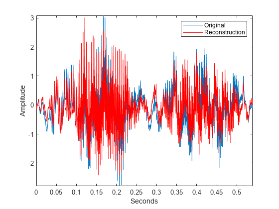
Plot the original and reconstructed signals.

plot(t,mtlb)
xlabel("Seconds")
ylabel("Amplitude")
hold on
plot(t,xrec,"r")
hold off
axis tight
legend("Original","Reconstruction")

Figure contains an axes object. The axes object with xlabel Seconds, ylabel Amplitude contains 2 objects of type line. These objects represent Original, Reconstruction.

If your computer has a sound card, you can listen to the original and reconstructed signals.

% To play the original signal, uncomment the next two lines
% p = audioplayer(mtlb,Fs);
% play(p)

% To play the reconstructed signal, uncomment the next two lines
% px = audioplayer(xrec,Fs);
% play(px)

Reconstruct a frequency-localized approximation to the Kobe earthquake data by extracting information from the CWT. The sampling frequency is 1 Hz. The extracted information corresponds to frequencies in the range [0.030 0.070] Hz.

load kobe

Obtain the CWT. Then, obtain the inverse CWT and add the signal mean back into the reconstructed data. The CWT does not preserve the signal mean.

[cfs,f] = cwt(kobe,1);
xrec = icwt(cfs,[],f,[0.030 0.070],SignalMean=mean(kobe));

Plot the original and reconstructed data.

subplot(2,1,1)
plot(kobe)
grid on
title("Original Data")
ylabel("Amplitude")
axis tight

subplot(2,1,2)
plot(xrec)
grid on
title("Bandpass Filtered Reconstruction [0.030 0.070] Hz");
xlabel("Time (s)")
ylabel("Amplitude")
axis tight

Figure contains 2 axes objects. Axes object 1 with title Original Data, ylabel Amplitude contains an object of type line. Axes object 2 with title Bandpass Filtered Reconstruction [0.030 0.070] Hz, xlabel Time (s), ylabel Amplitude contains an object of type line.

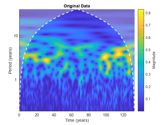
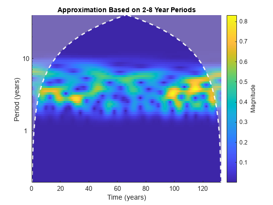
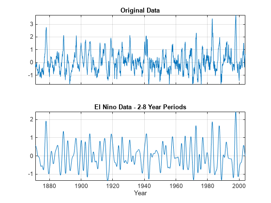
Use the inverse continuous wavelet transform to reconstruct an approximation to El Nino data based on 2 to 8 year periods.

Load the El Nino data and obtain its CWT. The data is sampled monthly. To obtain the periods in years, specify the sampling interval as 1/12 of a year.

load ninoairdata
[cfs,period] = cwt(nino,years(1/12));

Obtain the inverse CWT for periods of 2 to 8 years.

xrec = icwt(cfs,[],period,[years(2) years(8)]);

Plot the CWT of the reconstructed data and compare it to the CWT of the original data.

cwt(nino,years(1/12))
title("Original Data")

Figure contains an axes object. The axes object with title Original Data, xlabel Time (years), ylabel Period (years) contains 3 objects of type image, line, area.

figure
cwt(xrec,years(1/12))
title("Approximation Based on 2-8 Year Periods")

Figure contains an axes object. The axes object with title Approximation Based on 2-8 Year Periods, xlabel Time (years), ylabel Period (years) contains 3 objects of type image, line, area.

Compare the original data with the reconstructed data in time.

figure
subplot(2,1,1)
plot(datayear,nino) 
grid on
ax = gca;
ax.XTickLabel = '';
axis tight
title("Original Data")

subplot(2,1,2)
plot(datayear,xrec) 
grid on
axis tight
xlabel("Year")
title("El Nino Data - 2-8 Year Periods")

Figure contains 2 axes objects. Axes object 1 with title Original Data contains an object of type line. Axes object 2 with title El Nino Data - 2-8 Year Periods, xlabel Year contains an object of type line.

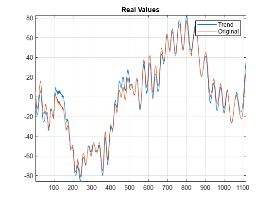
Add a trend to the continuous wavelet transform of a complex-valued dataset and reconstruct.

Obtain the CWT of the NPG2006 dataset.

load npg2006.mat
cfs = cwt(npg2006.cx);

Create a time-varying trend derived from the data.

trend = smoothdata(npg2006.cx,"movmean",100);

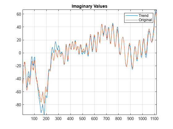
Obtain the inverse CWT and add the trend. Plot the original data and the reconstructed data.

xrec = icwt(cfs,SignalMean=trend);
plot([real(xrec)' real(npg2006.cx)])
grid on
title("Real Values")
legend("Trend","Original")
axis tight

Figure contains an axes object. The axes object with title Real Values contains 2 objects of type line. These objects represent Trend, Original.

figure
plot([imag(xrec)' imag(npg2006.cx)])
grid on
title("Imaginary Values")
legend("Trend","Original")
axis tight

Figure contains an axes object. The axes object with title Imaginary Values contains 2 objects of type line. These objects represent Trend, Original.

Load an ECG waveform. Create a CWT filter bank with periodic boundary handling that you can apply to the waveform.

load wecg
fb = cwtfilterbank(SignalLength=length(wecg),Boundary="periodic");

Obtain the two-sided frequency responses for the wavelet and scaling filters in the filter bank.

psif = freqz(fb,FrequencyRange="twosided",IncludeLowpass=true);

Use the filter bank to obtain the CWT of the waveform. Also obtain the scaling coefficients for the transform.

[cfs,~,~,scalcfs] = wt(fb,wecg);

Use the analysis filter bank to reconstruct the input. The approximate synthesis filters, or dual frame, are used to invert the transform.

xrecAN = icwt(cfs,[],ScalingCoefficients=scalcfs,...
    AnalysisFilterBank=psif);

Reconstruct the input using the default Morlet single integral formula.

xrecSI = icwt(cfs,[],ScalingCoefficients=scalcfs);

Compare the maximum reconstruction errors.

errAN = norm(xrecAN'-wecg,Inf)
errAN = 
6.6613e-16
errSI = norm(xrecSI'-wecg,Inf)
errSI = 
0.4037

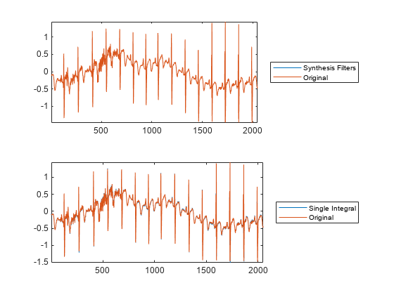
Plot both reconstructions.

subplot(2,1,1)
plot([xrecAN' wecg])
axis tight
    legend("Synthesis Filters","Original",Location="eastoutside")
subplot(2,1,2)
plot([xrecSI' wecg])
axis tight
legend("Single Integral","Original",Location="eastoutside")

Figure contains 2 axes objects. Axes object 1 contains 2 objects of type line. These objects represent Synthesis Filters, Original. Axes object 2 contains 2 objects of type line. These objects represent Single Integral, Original.

Input Arguments

collapse all

Continuous wavelet transform coefficients, specified as a matrix of complex values. cfs is the output from the cwt function.

If cfs is a 2-D matrix, icwt assumes that the CWT was obtained from a real-valued signal. If cfs is a 3-D matrix, icwt assumes that the CWT was obtained from a complex-valued signal. For a 3-D matrix, the first page of the cfs is the CWT of the positive (counterclockwise) component and the second page of cfs is the negative (clockwise) component. The pages represent the analytic and anti-analytic parts of the CWT, respectively.

Data Types: single | double
Complex Number Support: Yes

Analytic wavelet used to invert the CWT, specified as one of these:

  • "morse" — Morse wavelet

  • "amor" — Morlet wavelet

  • "bump" — bump wavelet

The specified wavelet must be the same wavelet used to obtain the CWT. The default Morse wavelet uses a symmetry parameter, γ, that is 3 and a time bandwidth of 60.

CWT frequencies, specified as a vector. The number of elements in the frequency vector must equal to the number of rows in the input CWT coefficient matrix, cfs. If you specify f, you must also specify freqrange.

Data Types: single | double

Frequency range for which to return inverse continuous wavelet transform values, specified as a two-element vector or 2-by-2 matrix.

  • If cfs is a 2-D matrix, freqrange must be a two-element vector.

  • If cfs is a 3-D matrix, freqrange can be a two-element vector or a 2-by-2 matrix.

    • If freqrange is a vector, icwt inverts the CWT over the same frequency range in both the positive (analytic) and negative (anti-analytic) components of cfs.

    • If freqrange is a 2-by-2 matrix, the first row contains the frequency range for the positive part of cfs (first page) and the second row contains the frequency range for the negative part of cfs (second page).

For a vector, the elements of freqrange must be strictly increasing and contained in the range of the frequency vector f. For a matrix, each row of freqrange must be strictly increasing and contained in the range of f. f is the scale-to-frequency conversion obtained in CWT. For the inversion of a complex-valued signal, you can specify one row of freqrange as a vector of zeros. If the first row of freqrange is a vector of zeros, only the negative (anti-analytic part) is used in the inversion.

If you specify freqrange, you must also specify f.

For example [0 0; 1/10 1/4] inverts the negative (clockwise) component over the frequency range [1/10 1/4]. The positive (counterclockwise) component is first set to all zeros before performing the inversion. Similarly, [1/10 1/4; 0 0] inverts the CWT by selecting the frequency range [1/10 1/4] from the positive (counterclockwise) component and setting the negative component to all zeros.

Data Types: single | double

Time periods corresponding to the rows of CWT coefficient matrix cfs, specified as a vector. period is the output of cwt, when the CWT is obtained using a duration input.

Data Types: duration

Period range for which to return inverse continuous wavelet transform values, specified as a two-element vector or 2-by-2 matrix.

  • If cfs is a 2-D matrix, periodrange must be a two-element vector of durations.

  • If cfs is a 3-D matrix, periodrange can be a two-element vector of durations or 2-by-2 matrix of durations.

    • If periodrange is a vector of durations, icwt inverts the CWT over the same frequency range in both the positive (analytic) and negative (anti-analytic) components of cfs.

    • If periodrange is a 2-by-2 matrix of durations, the first row contains the period range for the positive part of cfs (first page) and the second row contains the period range for the negative part of cfs (second page).

For a vector, the elements of periodrange must be strictly increasing and contained in the range of the period vector period. The elements of periodrange and period must have the same units. For a matrix, each row of periodrange must be strictly increasing and contained in the range of the period vector P. For the inversion of a complex-valued signal, you can specify one row of periodrange as a vector of zero durations. If the first row of periodrange is a vector of zero durations, only the negative (anti-analytic part) is used in the inversion.

If you specify periodrange, you must also specify period.

For example [seconds(0) seconds(0); seconds(1/10) seconds(1/4)] inverts the negative(clockwise) component over the period range [seconds(1/10) seconds(1/4)]. The positive (counterclockwise) component is first set to all zeros before performing the inversion. Similarly, [seconds(1/10) seconds(1/4); seconds(0) seconds(0)] inverts the CWT by selecting the period range [1/10 1/4] from the positive (counterclockwise) component and setting the negative component to all zeros.

Data Types: duration

Name-Value Arguments

Specify optional pairs of arguments as Name1=Value1,...,NameN=ValueN, where Name is the argument name and Value is the corresponding value. Name-value arguments must appear after other arguments, but the order of the pairs does not matter.

Example: xrec = icwt(cfs,"bump",VoicesPerOctave=10) returns the inverse CWT of cfs using the bump wavelet and 10 voices per octave.

Before R2021a, use commas to separate each name and value, and enclose Name in quotes.

Example: xrec = icwt(cfs,"WaveletParameters",[3 40],"SignalMean",sigmean) inverts the CWT using the Morse (3,40) wavelet and signal mean sigmean.

Time bandwidth of the Morse wavelet, specified as a scalar greater than 3 and less than or equal to 120. The specified time bandwidth must be the same time-bandwidth value used in the cwt. The symmetry of the Morse wavelet is assumed to be 3.

If you specify TimeBandwidth, you cannot specify WaveletParameters.

This syntax is not valid if you specify the AnalysisFilterBank name-value argument.

Data Types: single | double

Symmetry and time bandwidth of Morse wavelet, specified as a two-element vector of scalars. The first element of the vector is the symmetry, γ, and the second element is the time-bandwidth. The specified wavelet parameters must be the same values used in the CWT.

If you specify WaveletParameters, you cannot specify TimeBandwidth.

This syntax is not valid if you specify the AnalysisFilterBank name-value argument.

Data Types: single | double

Signal mean to add to the icwt output, specified as a scalar or vector. If the signal mean is a vector, it must be the same length as the column size of the wavelet coefficient matrix cfs.

  • If cfs is a 2-D matrix, the signal mean must be a real-valued scalar or vector.

  • If cfs is a 3-D matrix, the signal mean must be a complex-valued scalar or vector.

Because cwt does not preserve the signal mean, the inverse CWT is a zero-mean signal by default. Adding a non-zero signal mean to a frequency- or period-limited reconstruction adds a zero-frequency component to the reconstruction.

This syntax is not valid if you specify the AnalysisFilterBank name-value argument.

Data Types: single | double
Complex Number Support: Yes

Scaling coefficients to use in the inverse CWT, specified as a real- or complex-valued vector, obtained as an optional output of cwt. The length of ScalingCoefficients is equal to the column size of cfs.

  • If you only specify ScalingCoefficients without the AnalysisFilterBank name-value argument, the single-integral approximation is used to obtain the inverse CWT.

  • If you specify ScalingCoefficients with the AnalysisFilterBank name-value argument, the synthesis filters are used to obtain the inverse CWT.

You cannot specify both SignalMean and ScalingCoefficients name-value arguments.

Data Types: single | double
Complex Number Support: Yes

Bank of analysis filters used in inverting the CWT, specified as a matrix. The approximate synthesis filters, or dual frame, are used in the inversion. In most cases, use of the approximate synthesis filters results in a more accurate signal reconstruction. The wavelet name input is ignored if you specify the analysis filters.

To use the analysis filters, you must obtain the CWT with ExtendSignal set to false in cwt, or equivalently, Boundary set to "periodic" in cwtfilterbank. Obtain the analysis filters from the freqz object function of the filter bank with FrequencyRange="twosided" and IncludeLowpass=true.

Data Types: single | double

Number of voices per octave used in inverting the CWT, specified as an integer from 1 to 48. The CWT scales are discretized using the specified number of voices per octave. The number of voices per octave must be the same value used to obtain the CWT.

You cannot specify the number of voices per octave if you specify either the frequency, f, or duration, period. This syntax is not valid if you specify the AnalysisFilterBank name-value argument.

Data Types: single | double

Output Arguments

collapse all

Inverse 1-D continuous wavelet transform, returned as a real- or complex-valued row vector.

Data Types: single | double
Complex Number Support: Yes

More About

collapse all

Inverse Continuous Wavelet Transform — Single Integral Formula

By default, icwt computes the inverse CWT based on a discretized version of the single integral formula due to Morlet [5]. For a brief description of the theoretical foundation for the single integral formula, see Inverse Continuous Wavelet Transform. For additional theoretical information, see section 2.4 of [6]. The discretized version of this integral is presented in [7].

References

[1] Lilly, J. M., and S. C. Olhede. "Generalized Morse Wavelets as a Superfamily of Analytic Wavelets." IEEE Transactions on Signal Processing 60, no. 11 (November 2012): 6036–41. https://doi.org/10.1109/TSP.2012.2210890.

[2] Lilly, J.M., and S.C. Olhede. "Higher-Order Properties of Analytic Wavelets." IEEE Transactions on Signal Processing 57, no. 1 (January 2009): 146–60. https://doi.org/10.1109/TSP.2008.2007607.

[3] Lilly, J. M. jLab: A data analysis package for MATLAB®, version 1.6.2. 2016. http://www.jmlilly.net/jmlsoft.html.

[4] Lilly, J. M., and J.-C. Gascard. "Wavelet Ridge Diagnosis of Time-Varying Elliptical Signals with Application to an Oceanic Eddy." Nonlinear Processes in Geophysics 13, no. 5 (September 14, 2006): 467–83. https://doi.org/10.5194/npg-13-467-2006.

[5] Duval-Destin, M., M. A. Muschietti, and B. Torresani. “Continuous Wavelet Decompositions, Multiresolution, and Contrast Analysis.” SIAM Journal on Mathematical Analysis 24, no. 3 (May 1993): 739–55. https://doi.org/10.1137/0524045.

[6] Daubechies, Ingrid. Ten Lectures on Wavelets. CBMS-NSF Regional Conference Series in Applied Mathematics 61. Philadelphia, Pa: Society for Industrial and Applied Mathematics, 1992.

[7] Torrence, Christopher, and Gilbert P. Compo. “A Practical Guide to Wavelet Analysis.” Bulletin of the American Meteorological Society 79, no. 1 (January 1, 1998): 61–78. https://doi.org/10.1175/1520-0477(1998)079<0061:APGTWA>2.0.CO;2.

[8] Holschneider, M., and Ph. Tchamitchian. “Pointwise Analysis of Riemann’s 'Nondifferentiable' Function.” Inventiones Mathematicae 105, no. 1 (December 1991): 157–75. https://doi.org/10.1007/BF01232261.
Extended Capabilities

C/C++ Code Generation
Generate C and C++ code using MATLAB® Coder™.

Version History

Introduced in R2016b

expand all