CWT-Based Time-Frequency Analysis

Time-Frequency Analysis of Modulated Signals

Load a quadratic chirp signal. Use the helper function helperCWTTimeFreqPlot to show a plot of its spectrogram. The signal's frequency begins at approximately 500 Hz at t = 0, decreases to 100 Hz at t=2, and increases back to 500 Hz at t=4. The sampling frequency is 1 kHz. The code for the helper function is in the same directory as this example file.

load quadchirp
fs = 1000;
[S,F,T] = spectrogram(quadchirp,100,98,128,fs);
helperCWTTimeFreqPlot(S,T,F, ...
    'surf','STFT of Quadratic Chirp','Seconds','Hz')

Obtain a time-frequency plot of this signal using the CWT.

[cfs,f] = cwt(quadchirp,fs,'WaveletParameters',[14,200]);
helperCWTTimeFreqPlot(cfs,tquad,f, ...
    'surf','CWT of Quadratic Chirp','Seconds','Hz')

The CWT with the bump wavelet produces a time-frequency analysis very similar to the STFT.

Frequency and amplitude modulation occur frequently in natural signals. Use the CWT to obtain a time-frequency analysis of an echolocation pulse emitted by a big brown bat (Eptesicus Fuscus). The sampling interval is 7 microseconds. Use the bump wavelet with 32 voices per octave. Thanks to Curtis Condon, Ken White, and Al Feng of the Beckman Center at the University of Illinois for the bat data and permission to use it in this example.

load batsignal
t = 0:DT:(numel(batsignal)*DT)-DT;
[cfs,f] = cwt(batsignal,'bump',1/DT,'VoicesPerOctave',32);
helperCWTTimeFreqPlot(cfs,t*1e6,f./1000, ...
    'surf','CWT of Bat Echolocation','Microseconds','kHz')

Obtain and plot the STFT of the bat data.

[S,F,T] = spectrogram(batsignal,50,48,128,1/DT);
helperCWTTimeFreqPlot(S,T.*1e6,F./1e3, ...
    'surf','Bat Echolocation (STFT)','Microseconds','kHz')

For both the simulated and natural modulated signals, the CWT provides results similar to the STFT.

Detection of Transients in Oscillations Using the CWT

There are certain situations in time-frequency analysis where the CWT can provide a more informative time-frequency transform than the short-time Fourier transform. One such situation occurs when the signal is corrupted by transients. The appearance and disappearance of these transients often has physical significance. Therefore, it is important to be able to localize these transients in addition to characterizing oscillatory components in the signal. To simulate this, create a signal consisting of two sine waves with frequencies of 150 and 200 Hz. The sampling frequency is 1 kHz. The sine waves have disjoint time supports. The 150-Hz sine wave occurs between 100 and 300 milliseconds. The 200-Hz sine wave occurs from 700 milliseconds to 1 second. Additionally, there are two transients at 222 and 800 milliseconds. The signal is corrupted by noise.

rng default
dt = 0.001;
t = 0:dt:1-dt;
addNoise = 0.025*randn(size(t));
x = cos(2*pi*150*t).*(t>=0.1 & t<0.3)+sin(2*pi*200*t).*(t>0.7);
x = x+addNoise;
x([222 800]) = x([222 800 ])+[-2 2];
%figure;
plot(t.*1000,x)
xlabel('Milliseconds')
ylabel('Amplitude')

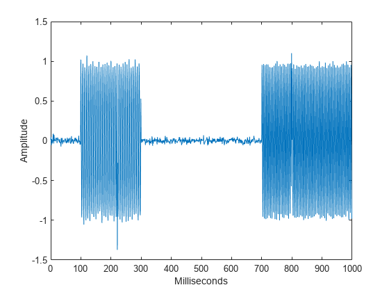
Zoom in on the two transients to see that they represent disturbances in the oscillations at 150 and 200 Hz.

subplot(2,1,1)
plot(t(184:264).*1000,x(184:264))
ylabel('Amplitude')
title('Transients')
axis tight
subplot(2,1,2)
plot(t(760:840).*1000,x(760:840))
ylabel('Amplitude')
axis tight
xlabel('Milliseconds')

Obtain and plot the CWT using the analytic Morlet wavelet.

figure
[cfs,f] = cwt(x,1/dt,'amor');
contour(t*1000,f,abs(cfs))
grid on
c = colorbar;
xlabel('Milliseconds')
ylabel('Frequency')
c.Label.String = 'Magnitude';

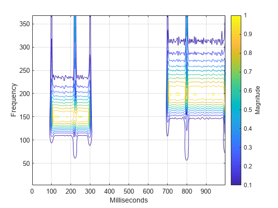
The analytic Morlet wavelet exhibits poorer frequency localization than the bump wavelet, but superior time localization. This makes the Morlet wavelet a better choice for transient localization. Plot the magnitude-squared fine scale coefficients to demonstrate the localization of the transients.

figure
wt = cwt(x,1/dt,'amor');
plot(t.*1000,abs(wt(1,:)).^2)
xlabel('Milliseconds')
ylabel('Magnitude')
grid on
title('Analytic Morlet Wavelet -- Fine Scale Coefficients');

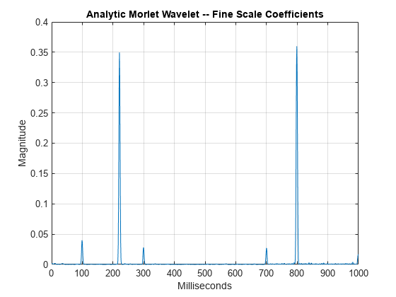
%hold off

The wavelet shrinks to enable time localization of the transients with a high degree of accuracy while stretching to permit frequency localization of the oscillations at 150 and 200 Hz.

The STFT can only localize the transients to the width of the window. You must plot the STFT in decibels (dB) to be able to visualize the transients.

[S,F,T] = spectrogram(x,50,48,128,1000);
surf(T.*1000,F,20*log10(abs(S)),'edgecolor','none')
view(0,90)
axis tight
shading interp
colorbar
xlabel('Time')
ylabel('Hz')
title('STFT')

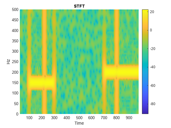
The transients appear in the STFT only as a broadband increase in power. Compare short-time power estimates obtained from the STFT before (centered at 183 msec) and after (centered at 223 msec) the appearance of the first transient.

figure
plot(F,20*log10(abs(S(:,80))))
hold on
plot(F,20*log10(abs(S(:,100))),'r')
hold off
legend('T = 183 msec','T = 223 msec')
xlabel('Hz')
ylabel('dB')

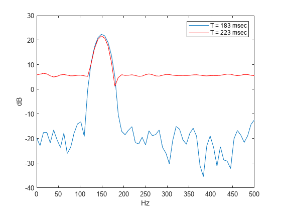
The STFT does not provide the ability to localize transients to the same degree as the CWT.

Removing A Time-Localized Frequency Component Using the Inverse CWT

Create a signal consisting of exponentially weighted sine waves. There are two 25-Hz components -- one centered at 0.2 seconds and one centered at 0.5 seconds. There are two 70-Hz components -- one centered at 0.2 and one centered at 0.8 seconds. The first 25-Hz and 70-Hz components co-occur in time.

t = 0:1/2000:1-1/2000;
dt = 1/2000;
x1 = sin(50*pi*t).*exp(-50*pi*(t-0.2).^2);
x2 = sin(50*pi*t).*exp(-100*pi*(t-0.5).^2);
x3 = 2*cos(140*pi*t).*exp(-50*pi*(t-0.2).^2);
x4 = 2*sin(140*pi*t).*exp(-80*pi*(t-0.8).^2);
x = x1+x2+x3+x4;
figure
plot(t,x)
title('Superimposed Signal')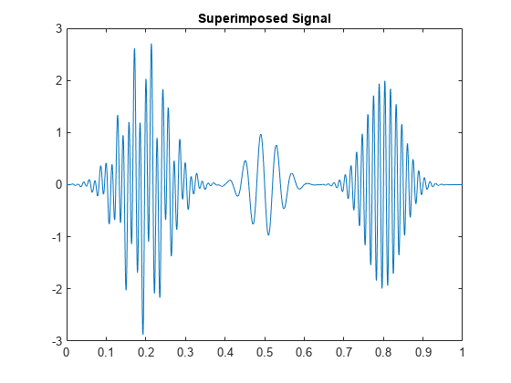

Obtain and display the CWT.

cwt(x,2000)
title('Analytic CWT using Default Morse Wavelet');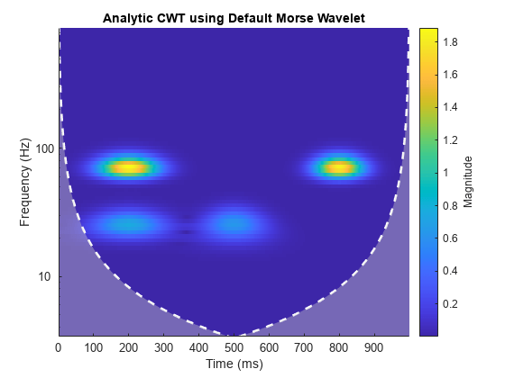

Remove the 25 Hz component which occurs from approximately 0.07 to 0.3 seconds by zeroing out the CWT coefficients. Use the inverse CWT (icwt) to reconstruct an approximation to the signal.

[cfs,f] = cwt(x,2000);
T1 = .07;  T2 = .33;
F1 = 19;   F2 = 34;
cfs(f > F1 & f < F2, t> T1 & t < T2) = 0;
xrec = icwt(cfs);

Display the CWT of the reconstructed signal. The initial 25-Hz component is removed.

cwt(xrec,2000)

Plot the original signal and the reconstruction.

subplot(2,1,1)
plot(t,x)
title('Original Signal')
subplot(2,1,2)
plot(t,xrec)
title('Signal with first 25-Hz component removed')

Finally, compare the reconstructed signal with the original signal without the 25-Hz component centered at 0.2 seconds.

y = x2+x3+x4;
figure
plot(t,xrec)
hold on
plot(t,y,'r--')
hold off
legend('Inverse CWT approximation','Original signal without 25-Hz')

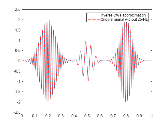
Determining Exact Frequency Through the Analytic CWT

When you obtain the wavelet transform of a sine wave using an analytic wavelet, the analytic CWT coefficients actually encode the frequency.

To illustrate this, consider an otoacoustic emission obtained from a human ear. Otoacoustic emissions (OAEs) are emitted by the cochlea (inner ear) and their presence are indicative of normal hearing. Load and plot the OAE data. The data are sampled at 20 kHz.

load dpoae
plot(t.*1000,dpoaets)
xlabel('Milliseconds')
ylabel('Amplitude')

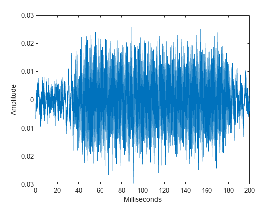
The emission was evoked by a stimulus beginning at 25 milliseconds and ending at 175 milliseconds. Based on the experimental parameters, the emission frequency should be 1230 Hz. Obtain and plot the CWT.

cwt(dpoaets,'bump',20000)
xlabel('Milliseconds')

You can investigate the time evolution of the OAE by finding the CWT coefficients closest in frequency to 1230 Hz and examining their magnitudes as a function of time. Plot the magnitudes along with time markers designating the beginning and end of the evoking stimulus.

[dpoaeCWT,f] = cwt(dpoaets,'bump',20000);
[~,idx1230] = min(abs(f-1230));
cfsOAE = dpoaeCWT(idx1230,:);
plot(t.*1000,abs(cfsOAE))
hold on
AX = gca;
plot([25 25],[AX.YLim(1) AX.YLim(2)],'r')
plot([175 175],[AX.YLim(1) AX.YLim(2)],'r')
hold off
xlabel('Milliseconds')
ylabel('Magnitude')
title('CWT Coefficient Magnitudes')

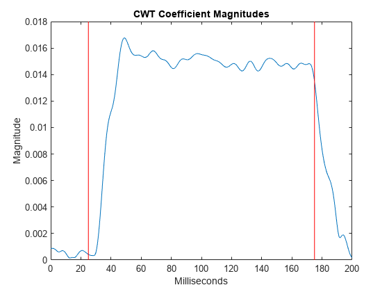
There is some delay between the onset of the evoking stimulus and the OAE. Once the evoking stimulus is terminated, the OAE immediately begins to decay in magnitude.

Another way to isolate the emission is to use the inverse CWT to reconstruct a frequency-localized approximation in the time domain.

Reconstruct a frequency-localized emission approximation by inverting the CWT in the frequency range [1150 1350] Hz. Plot the original data along with the reconstruction and markers indicating the beginning and end of the evoking stimulus.

xrec = icwt(dpoaeCWT,'bump',f,[1150 1350]);
%figure
plot(t.*1000,dpoaets)
hold on
plot(t.*1000,xrec,'r')
AX = gca;
ylim = AX.YLim;
plot([25 25],ylim,'k')
plot([175 175],ylim,'k')
hold off
xlabel('Milliseconds')
ylabel('Amplitude')
title('Frequency-Localized Reconstruction of Emission')

In the time-domain data, you clearly see how the emission ramps on and off at the application and termination of the evoking stimulus.

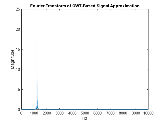
It is important to note that even though a range of frequencies were selected for the reconstruction, the analytic wavelet transform actually encodes the exact frequency of the emission. To demonstrate this, take the Fourier transform of the emission approximation reconstructed from the analytic CWT.

xdft = fft(xrec);
freq = 0:2e4/numel(xrec):1e4;
xdft = xdft(1:numel(xrec)/2+1);
figure
plot(freq,abs(xdft))
xlabel('Hz')
ylabel('Magnitude')
title('Fourier Transform of CWT-Based Signal Approximation')

[~,maxidx] = max(abs(xdft));
fprintf('The frequency is %4.2f Hz.\n',freq(maxidx));

The frequency is 1230.00 Hz.

Conclusions

In this example you learned how to use the CWT to obtain a time-frequency analysis of a 1-D signal using an analytic wavelet with cwt. You saw examples of signals where the CWT provides similar results to the STFT and an example where the CWT can provide more interpretable results than the STFT. Finally, you learned how to reconstruct time-scale (frequency) localized approximations to a signal using icwt.

References

[1] Mallat, S. G. A Wavelet Tour of Signal Processing: The Sparse Way. 3rd ed. Amsterdam ; Boston: Elsevier/Academic Press, 2009.