Time-Frequency Analysis and Continuous Wavelet Transform

Load Hyperbolic Chirp

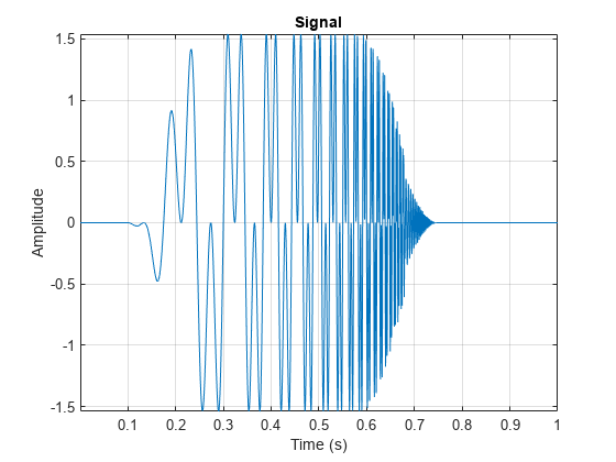
Load a signal that has two hyperbolic chirps. The data are sampled at 2048 Hz. The first chirp is active between 0.1 and 0.68 seconds, and the second chirp is active between 0.1 and 0.75 seconds. The instantaneous frequency (in hertz) of the first chirp at time $$t$$ is $$\frac{15\pi }{{(0.8-t)}^2}/2\pi$$. The instantaneous frequency of the second chirp at time $$t$$ is $$\frac{5\pi }{{(0.8-t)}^2}/2\pi$$. Plot the signal.

load hychirp
plot(t,hychirp)
grid on
title("Signal")
axis tight
xlabel("Time (s)")
ylabel('Amplitude')

Time-Frequency Analysis: Fourier Transform

The Fourier transform (FT) is very good at identifying frequency components present in a signal. However, the FT does not identify when the frequency components occur.

Plot the magnitude spectrum of the signal. Zoom in on the region between 0 and 200 Hz.

sigLen = numel(hychirp);
fchirp = fft(hychirp);
fr = Fs*(0:1/Fs:1-1/Fs);
plot(fr(1:sigLen/2),abs(fchirp(1:sigLen/2)),"x-")
xlabel("Frequency (Hz)")
ylabel("Amplitude")
axis tight
grid on
xlim([0 200])

Time-Frequency Analysis: Short-Time Fourier Transform

The Fourier transform does not provide time information. To determine when the changes in frequency occur, the short-time Fourier transform (STFT) approach segments the signal into different chunks and performs the FT on each chunk. The STFT tiling in the time-frequency plane is shown here.

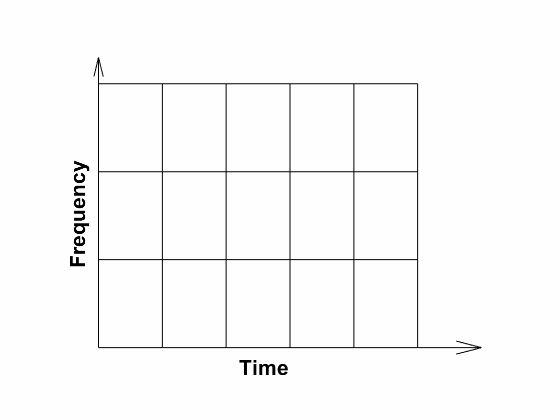
The STFT provides some information on both the timing and the frequencies at which a signal event occurs. However, choosing a window (segment) size is key. For time-frequency analysis using the STFT, choosing a shorter window size helps obtain good time resolution at the expense of frequency resolution. Conversely, choosing a larger window helps obtain good frequency resolution at the expense of time resolution.

Once you pick a window size, it remains fixed for the entire analysis. If you can estimate the frequency components you are expecting in your signal, then you can use that information to pick a window size for the analysis.

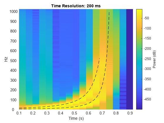
The instantaneous frequencies of the two chirps at their initial time points are approximately 5 Hz and 15 Hz. Use the helper function helperPlotSpectrogram to plot the spectrogram of the signal with a time window size of 200 milliseconds. The source code for helperPlotSpectrogram is listed in the appendix. The helper function plots the instantaneous frequencies over the spectrogram as black dashed-line segments. The instantaneous frequencies are resolved early in the signal, but not as well later.

helperPlotSpectrogram(hychirp,t,Fs,200)

Now use helperPlotSpectrogram to plot the spectrogram with a time window size of 50 milliseconds. The higher frequencies, which occur later in the signal, are now resolved, but the lower frequencies at the beginning of the signal are not.

helperPlotSpectrogram(hychirp,t,Fs,50)

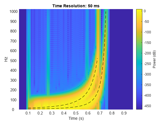
For nonstationary signals like the hyperbolic chirp, using the STFT is problematic. No single window size can resolve the entire frequency content of such signals.

Time-Frequency Analysis: Continuous Wavelet Transform

The continuous wavelet transform (CWT) was created to overcome the resolution issues inherent in the STFT. The CWT tiling on the time-frequency plane is shown here.

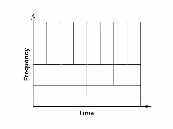
The CWT tiling of the plane is useful because many real-world signals have slowly oscillating content that occurs on long scales, while high frequency events tend to be abrupt or transient. However, if it were natural for high-frequency events to be long in duration, then using the CWT would not be appropriate. You would have poorer frequency resolution without gaining any time resolution. But that is quite often not the case. The human auditory system works this way; we have much better frequency localization at lower frequencies, and better time localization at high frequencies.

Plot the scalogram of the CWT. The scalogram is the absolute value of the CWT plotted as a function of time and frequency. The plot uses a logarithmic frequency axis because frequencies in the CWT are logarithmic. The presence of the two hyperbolic chirps in the signal is clear from the scalogram. With the CWT, you can accurately estimate the instantaneous frequencies throughout the duration of the signal, without worrying about picking a segment length.

cwt(hychirp,Fs)

The white dashed line marks what is known as the cone of influence. The cone of influence shows areas in the scalogram potentially affected by boundary effects. For more information, see Boundary Effects and the Cone of Influence.

To get a sense of how rapidly the magnitude of the wavelet coefficients grows, use the helper function helperPlotScalogram3d to plot the scalogram as a 3-D surface. The source code for helperPlotScalogram3d is listed in the appendix.

helperPlotScalogram3d(hychirp,Fs)

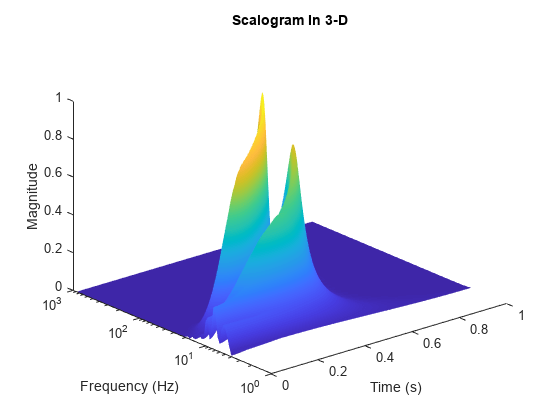
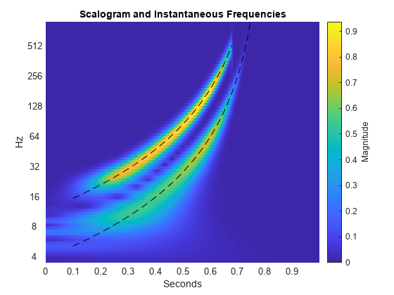
Use the helper function helperPlotScalogram to plot the scalogram of the signal and the instantaneous frequencies. The source code for helperPlotScalogram is listed in the appendix. The instantaneous frequencies align well with the scalogram features.

helperPlotScalogram(hychirp,Fs)

Appendix – Helper Functions

helperPlotSpectrogram

function helperPlotSpectrogram(sig,t,Fs,timeres)
% This function is only intended to support this wavelet example.
% It may change or be removed in a future release.

[px,fx,tx] = pspectrum(sig,Fs,"spectrogram",TimeResolution=timeres/1000);
hp = pcolor(tx,fx,20*log10(abs(px)));
hp.EdgeAlpha = 0;
ylims = hp.Parent.YLim;
yticks = hp.Parent.YTick;
cl = colorbar;
cl.Label.String = "Power (dB)";
axis tight
hold on
title("Time Resolution: "+num2str(timeres)+" ms")
xlabel("Time (s)")
ylabel("Hz");
dt  = 1/Fs;
idxbegin = round(0.1/dt);
idxend1 = round(0.68/dt);
idxend2 = round(0.75/dt);
instfreq1 = abs((15*pi)./(0.8-t).^2)./(2*pi);
instfreq2 = abs((5*pi)./(0.8-t).^2)./(2*pi);
plot(t(idxbegin:idxend1),(instfreq1(idxbegin:idxend1)),'k--');
hold on;
plot(t(idxbegin:idxend2),(instfreq2(idxbegin:idxend2)),'k--');
ylim(ylims);
hp.Parent.YTick = yticks;
hp.Parent.YTickLabels = yticks;
hold off
end

helperPlotScalogram

function helperPlotScalogram(sig,Fs)
% This function is only intended to support this wavelet example.
% It may change or be removed in a future release.
[cfs,f] = cwt(sig,Fs);

sigLen = numel(sig);
t = (0:sigLen-1)/Fs;

hp = pcolor(t,log2(f),abs(cfs));
hp.EdgeAlpha = 0;
ylims = hp.Parent.YLim;
yticks = hp.Parent.YTick;
cl = colorbar;
cl.Label.String = "Magnitude";
axis tight
hold on
title("Scalogram and Instantaneous Frequencies")
xlabel("Seconds");
ylabel("Hz");
dt  = 1/2048;
idxbegin = round(0.1/dt);
idxend1 = round(0.68/dt);
idxend2 = round(0.75/dt);
instfreq1 = abs((15*pi)./(0.8-t).^2)./(2*pi);
instfreq2 = abs((5*pi)./(0.8-t).^2)./(2*pi);
plot(t(idxbegin:idxend1),log2(instfreq1(idxbegin:idxend1)),"k--");
hold on;
plot(t(idxbegin:idxend2),log2(instfreq2(idxbegin:idxend2)),"k--");
ylim(ylims);
hp.Parent.YTick = yticks;
hp.Parent.YTickLabels = 2.^yticks;
end

helperPlotScalogram3d

function helperPlotScalogram3d(sig,Fs)
% This function is only intended to support this wavelet example.
% It may change or be removed in a future release.
figure
[cfs,f] = cwt(sig,Fs);

sigLen = numel(sig);
t = (0:sigLen-1)/Fs;
surface(t,f,abs(cfs));
xlabel("Time (s)")
ylabel("Frequency (Hz)")
zlabel("Magnitude")
title("Scalogram In 3-D")
set(gca,Yscale="log")
shading interp
view([-40 30])
end