wcoherence

Wavelet coherence and cross-spectrum

Syntax

wcoh = wcoherence(x,y)

[wcoh,wcs]
= wcoherence(x,y)

[wcoh,wcs,period]
= wcoherence(x,y,ts)

 [wcoh,wcs,f]
= wcoherence(x,y,fs)

[wcoh,wcs,f,coi]
= wcoherence(___)

 [wcoh,wcs,period,coi]
= wcoherence(___,ts)

[___,coi,wtx,wty] = wcoherence(___)

[___] = wcoherence(___,Name=Value)

wcoherence(___)

Description

wcoh = wcoherence(x,y) returns the magnitude-squared wavelet coherence, which is a measure of the correlation between signals x and y in the time-frequency plane. Wavelet coherence is useful for analyzing nonstationary signals. The inputs x and y must be equal length, 1-D, real-valued signals. The coherence is computed using the analytic Morlet wavelet.

example

[wcoh,wcs] = wcoherence(x,y) returns the smoothed wavelet cross spectrum of x and y. You can use the phase of the cross spectrum values to identify the relative lag between the input signals.

[wcoh,wcs,period] = wcoherence(x,y,ts) uses the positive duration ts as the sampling interval. The duration ts is used to compute the scale-to-period conversion, period. The duration array period has the same format as specified in ts.

example

[wcoh,wcs,f] = wcoherence(x,y,fs) uses the positive sampling frequency, fs, to compute the scale-to-frequency conversion, f. The sampling frequency fs is in Hz.

example

[wcoh,wcs,f,coi] = wcoherence(___) returns the cone of influence, coi, for the wavelet coherence in cycles per sample. If you specify the sampling frequency, fs, the cone of influence is in Hz.

[wcoh,wcs,period,coi] = wcoherence(___,ts) returns the cone of influence, coi, in cycles per unit time.

example

[___,coi,wtx,wty] = wcoherence(___) returns the continuous wavelet transforms (CWT) of x and y in wtx, wty, respectively. wtx and wty are used in the formation of the wavelet cross spectrum and coherence estimates.

[___] = wcoherence(___,Name=Value) specifies options using one or more name-value arguments in addition to the input arguments in previous syntaxes.

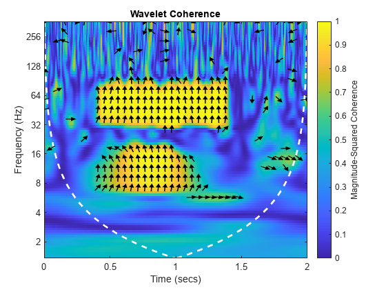
wcoherence(___) with no output arguments plots the wavelet coherence and cone of influence in the current figure. Due to the inverse relationship between frequency and period, a plot that uses the sampling interval is the inverse of a plot the uses the sampling frequency. For areas where the coherence exceeds 0.5, plots that use the sampling frequency display arrows to show the phase lag of y with respect to x. The arrows are spaced in time and scale. The direction of the arrows corresponds to the phase lag on the unit circle. For example, a vertical arrow indicates a π/2 or quarter-cycle phase lag. The corresponding lag in time depends on the duration of the cycle.

example

Examples

collapse all

Wavelet Coherence of Two Sine Waves

Open Live Script

Use default wcoherence settings to obtain the wavelet coherence between a sine wave with random noise and a frequency-modulated signal with decreasing frequency over time.

t  = linspace(0,1,1024);
x = -sin(8*pi*t) + 0.4*randn(1,1024);
x = x/max(abs(x));
y = wnoise("doppler",10);
wcoh = wcoherence(x,y);

The default coherence computation uses the analytic Morlet wavelet, 12 voices per octave and smooths 12 scales. The default number of octaves is equal to floor(log2(numel(x)))-1, which in this case is 9.

Effect of Sampling Interval on Wavelet Coherence

Open Live Script

Obtain the wavelet coherence data for two signals, specifying a sampling interval of 0.001 seconds. Both signals consist of two sine waves (10 Hz and 50 Hz) in white noise. The sine waves have different time supports.

Set the random number generator to its default settings for reproducibility. Then create the two signals.

rng default
t = 0:0.001:2;
x = cos(2*pi*10*t).*(t>=0.5 & t<1.1)+ ...
    cos(2*pi*50*t).*(t>= 0.2 & t< 1.4)+ ...
    0.25*randn(size(t));
y = sin(2*pi*10*t).*(t>=0.6 & t<1.2)+ ...
    sin(2*pi*50*t).*(t>= 0.4 & t<1.6)+ ...
    0.35*randn(size(t));
tiledlayout(2,1)
nexttile
plot(t,x)
title("X")
nexttile
plot(t,y)
title("Y")
xlabel("Time (seconds)")

Figure contains 2 axes objects. Axes object 1 with title X contains an object of type line. Axes object 2 with title Y, xlabel Time (seconds) contains an object of type line.

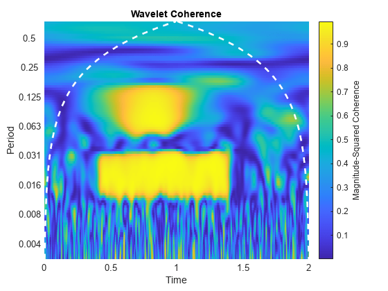
Obtain the coherence of the two signals. Also obtain the scale-to-period conversion and cone of influence.

[wcoh,~,period,coi] = wcoherence(x,y,seconds(0.001));

Use the pcolor command to plot the coherence and cone of influence.

figure
period = seconds(period);
coi = seconds(coi);
h = pcolor(t,log2(period),wcoh);
h.EdgeColor = "none";
ax = gca;
ytick=round(pow2(ax.YTick),3);
ax.YTickLabel=ytick;
ax.XLabel.String="Time";
ax.YLabel.String="Period";
ax.Title.String = "Wavelet Coherence";
hcol = colorbar;
hcol.Label.String = "Magnitude-Squared Coherence";
hold on
plot(ax,t,log2(coi),"w--",linewidth=2)
hold off

Figure contains an axes object. The axes object with title Wavelet Coherence, xlabel Time, ylabel Period contains 2 objects of type surface, line.

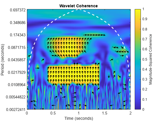
Use wcoherence(x,y,seconds(0.001)) without any output arguments. This plot includes the phase arrows and the cone of influence.

wcoherence(x,y,seconds(0.001))

Figure contains an axes object. The axes object with title Wavelet Coherence, xlabel Time (seconds), ylabel Period (seconds) contains 242 objects of type image, line, patch.

Effect of Sampling Frequency on Wavelet Coherence

Open Live Script

Obtain the wavelet coherence for two signals, specifying a sampling frequency of 1000 Hz. Both signals consist of two sine waves (10 Hz and 50 Hz) in white noise. The sine waves have different time supports.

Set the random number generator to its default settings for reproducibility and create the two signals.

rng default
t = 0:0.001:2;
x = cos(2*pi*10*t).*(t>=0.5 & t<1.1)+ ...
    cos(2*pi*50*t).*(t>= 0.2 & t< 1.4)+ ...
    0.25*randn(size(t));
y = sin(2*pi*10*t).*(t>=0.6 & t<1.2)+ ...
    sin(2*pi*50*t).*(t>= 0.4 & t<1.6)+ ...
    0.35*randn(size(t));

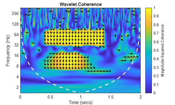
Obtain the wavelet coherence. The coherence plot is flipped with respect to the plot in the previous example, which specifies a sampling interval instead of a sampling frequency.

wcoherence(x,y,1000)

Figure contains an axes object. The axes object with title Wavelet Coherence, xlabel Time (secs), ylabel Frequency (Hz) contains 242 objects of type image, line, patch.

Effect of Number of Smoothed Scales on Wavelet Coherence

Open Live Script

Obtain the wavelet coherence for two signals sampled at 1000 Hz. Both signals consist of two sine waves (10 Hz and 50 Hz) in white noise. Use the default number of scales to smooth. This value is equivalent to the number of voices per octave. Both values default to 12.

Set the random number generator to its default settings for reproducibility. Then, create the two signals and obtain the coherence.

rng default
Fs = 1000;
t = 0:1/Fs:2;
x = cos(2*pi*10*t).*(t>=0.5 & t<1.1)+ ...
    cos(2*pi*50*t).*(t>= 0.2 & t< 1.4)+ ...
    0.25*randn(size(t));
y = sin(2*pi*10*t).*(t>=0.6 & t<1.2)+ ...
    sin(2*pi*50*t).*(t>= 0.4 & t<1.6)+ ...
    0.35*randn(size(t));
wcoherence(x,y,Fs)

Figure contains an axes object. The axes object with title Wavelet Coherence, xlabel Time (secs), ylabel Frequency (Hz) contains 242 objects of type image, line, patch.

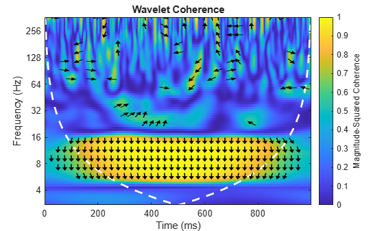
Set the number of scales to smooth to 18. The increased smoothing causes reduced low frequency resolution.

wcoherence(x,y,Fs,NumScalesToSmooth=18)

Figure contains an axes object. The axes object with title Wavelet Coherence, xlabel Time (secs), ylabel Frequency (Hz) contains 242 objects of type image, line, patch.

Effect of Phase Display Threshold on Wavelet Coherence of Weather Data

Open Live Script

Compare the effects of using different phase display thresholds on the wavelet coherence.

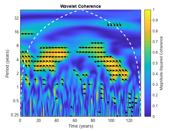
Plot the wavelet coherence between the El Nino time series and the All India Average Rainfall Index. The data are sampled monthly. Specify the sampling interval as 1/12 of a year to display the periods in years. Use the default phase display threshold of 0.5, which shows phase arrows only where the coherence is greater than or equal to 0.5.

load ninoairdata
wcoherence(nino,air,years(1/12))

Figure contains an axes object. The axes object with title Wavelet Coherence, xlabel Time (years), ylabel Period (years) contains 190 objects of type image, line, patch.

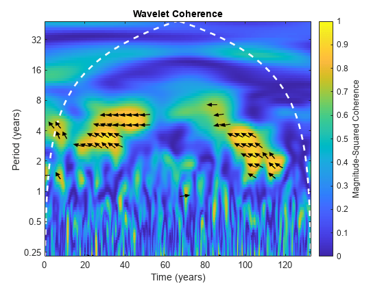
Set the phase display threshold to 0.7. Confirm the number of phase arrows decreases.

wcoherence(nino,air,years(1/12),PhaseDisplayThreshold=0.7);

Figure contains an axes object. The axes object with title Wavelet Coherence, xlabel Time (years), ylabel Period (years) contains 61 objects of type image, line, patch.

Input Arguments

collapse all

`x` — Input signal
vector of real values

Input signal, specified as a vector of real values. x must be a 1-D, real-valued signal. The two input signals, x and y, must be the same length and must have at least four samples.

`y` — Input signal
vector of real values

Input signal, specified as vector of real values. y must be a 1-D, real-valued signal. The two input signals, x and y, must be the same length and must have at least four samples.

`ts` — Sampling interval
duration with positive scalar input

Sampling interval, also known as the sampling period, specified as a duration with positive scalar input. Valid durations are years, days, hours, seconds, and minutes. You can also use the duration function to specify ts. You cannot use calendar durations (caldays, calweeks, calmonths, calquarters, or calyears).

You cannot specify both a sampling frequency fs and a sampling period ts.

`fs` — Sampling frequency
positive scalar | `[]`

Sampling frequency, specified as a positive scalar.

If you specify fs as empty, wcoherence uses normalized frequency in cycles/sample. The Nyquist frequency is ½.

You cannot specify both a sampling frequency fs and a sampling period ts.

Name-Value Arguments

Specify optional pairs of arguments as Name1=Value1,...,NameN=ValueN, where Name is the argument name and Value is the corresponding value. Name-value arguments must appear after other arguments, but the order of the pairs does not matter.

Example: wcoh = wcoherence(x,y,PhaseDisplayThreshold=0.7) specifies the threshold for displaying phase vectors.

Before R2021a, use commas to separate each name and value, and enclose Name in quotes.

Example: wcoh = wcoherence(x,y,"PhaseDisplayThreshold",0.7) specifies the threshold for displaying phase vectors.

`FrequencyLimits` — Frequency limits
two-element scalar vector

Frequency limits to use in wcoherence, specified as a two-element vector with positive strictly increasing elements.

The first element specifies the lowest peak passband frequency and must be greater than or equal to the product of the wavelet peak frequency in hertz and two time standard deviations divided by the signal length.
The second element specifies the highest peak passband frequency and must be less than or equal to the Nyquist frequency.

The base 2 logarithm of the ratio of the maximum frequency to the minimum frequency must be greater than or equal to 1/NV, where NV is the number of voices per octave.

If you specify frequency limits outside the permissible range, wcoherence truncates the limits to the minimum and maximum valid values. Use cwtfreqbounds with the wavelet set to "amor" to determine frequency limits for different parameterizations of the wavelet coherence.

Example: FrequencyLimits=[0.1 0.3]

`PeriodLimits` — Period limits
two-element duration array

Period limits to use in wcoherence, specified as a two-element duration array with strictly increasing positive elements. The first element must be greater than or equal to 2×ts, where ts is the sampling period. The base 2 logarithm of the ratio of the minimum period to the maximum period must be less than or equal to -1/NV, where NV is the number of voices per octave. The maximum period cannot exceed the signal length divided by the product of two time standard deviations of the wavelet and the wavelet peak frequency.

If you specify period limits outside the permissible range, wcoherence truncates the limits to the minimum and maximum valid values. Use cwtfreqbounds with the wavelet set to "amor" to determine period limits for different parameterizations of the wavelet coherence.

Example: PeriodLimits=[seconds(0.2) seconds(1)]

Data Types: duration

`VoicesPerOctave` — Number of voices per octave
12 (default) | even integer from 10 to 32

Number of voices per octave to use in the wavelet coherence, specified as an even integer from 10 to 32.

`NumScalesToSmooth` — Number of scales to smooth
positive integer

Number of scales to smooth in time and scale, specified as a positive integer less than or equal to one half N, where N is the number of scales in the wavelet transform. If unspecified, NumScalesToSmooth defaults to the minimum of floor(N/2) and VoicesPerOctave. The function uses a moving average filter to smooth across scale. If your coherence is noisy, you can specify a larger NumScalesToSmooth value to smooth the coherence more.

`NumOctaves` — Number of octaves
`floor(log2(numel(x)))-1` (default) | positive integer

Number of octaves to use in the wavelet coherence, specified as a positive integer between 1 and floor(log2(numel(x)))-1. If you do not need to examine lower frequency values, use a smaller NumOctaves value.

The NumOctaves name-value argument is not recommended and will be removed in a future release. The recommended way to modify the frequency or period range of wavelet coherence is with the 'FrequencyLimits' or 'PeriodLimits' name-value arguments. You cannot specify both the 'NumOctaves' and 'FrequencyLimits' or 'PeriodLimits' name-value arguments. See cwtfreqbounds.

`PhaseDisplayThreshold` — Threshold for displaying phase vectors
0.5 (default) | real scalar between 0 and 1

Threshold for displaying phase vectors, specified as a real scalar between 0 and 1. This function displays phase vectors for regions with coherence greater than or equal to the specified threshold value. Lowering the threshold value displays more phase vectors. If you use wcoherence with any output arguments, the PhaseDisplayThreshold value is ignored.

Output Arguments

collapse all

`wcoh` — Wavelet coherence
matrix

Wavelet coherence, returned as a matrix. The coherence is computed using the analytic Morlet wavelet over logarithmic scales, with a default value of 12 voices per octave. The default number of octaves is equal to floor(log2(numel(x)))-1. If you do not specify a sampling interval, sampling frequency is assumed.

For more information, see Wavelet Coherence.

`wcs` — Smoothed wavelet cross spectrum
matrix of complex values

Smoothed wavelet cross spectrum, returned as a matrix of complex values. You can use the phase of the cross spectrum values to identify the relative lag between the input signals.

For more information, see Smoothed Wavelet Cross Spectrum.

`period` — Scale-to-period conversion
array of durations

Scale-to-period conversion, returned as an array of durations. The conversion values are computed from the sampling period specified in ts. Each period element has the same format as ts.

`f` — Scale-to-frequency conversion
vector

Scale-to-frequency conversion, returned as a vector. The vector contains the peak frequency values for the wavelets used to compute the coherence. If you want to output f, but do not specify a sampling frequency input, fs, the returned wavelet coherence is in cycles per sample.

`coi` — Cone of influence
array of doubles | array of durations

Cone of influence for the wavelet coherence, returned as either an array of doubles or array of durations. The cone of influence indicates where edge effects occur in the coherence data. If you specify a sampling frequency, fs, the cone of influence is in Hz. If you specify a sampling interval or period, ts, the cone of influence is in periods. Due to the edge effects, give less credence to areas of apparent high coherence that are outside or overlap the cone of influence. The cone of influence is indicated by a dashed line.

For additional information, see Boundary Effects and the Cone of Influence.

`wtx` — Continuous wavelet transform of `x`
matrix

Continuous wavelet transform of x, returned as a matrix.

`wty` — Continuous wavelet transform of `y`
matrix

Continuous wavelet transform of y, returned as a matrix.

More About

collapse all

Smoothed Wavelet Cross Spectrum

The smoothed wavelet cross spectrum is a measure of the distribution of power of two signals.

The smoothed wavelet cross spectrum of two time series, x and y, is:

$C_{x y} (a, b) = S (C_{x} (a, b) C_{y}^{*} (a, b)),$

where C_x(a,b) and C_y(a,b) denote the continuous wavelet transforms of x and y at scales a and positions b. The superscript * is the complex conjugate, and S is a smoothing operator in time and scale.

For real-valued time series, the wavelet cross spectrum is real valued if you use a real-valued analyzing wavelet, and complex valued if you use a complex-valued analyzing wavelet.

Wavelet Coherence

Wavelet coherence is a measure of the correlation between two signals.

The wavelet coherence of two time series x and y is:

$\frac{{| S (C_{x} (a, b) C_{y}^{*} (a, b)) |}^{2}}{S (| C_{x} (a, b) |^{2}) \cdot S (| C_{y} (a, b) |^{2})},$

where C_x(a,b) and C_y(a,b) denote the continuous wavelet transforms of x and y at scales a and positions b. The superscript * is the complex conjugate and S is a smoothing operator in time and scale.

For real-valued time series, the wavelet coherence is real valued if you use a real-valued analyzing wavelet, and complex valued if you use a complex-valued analyzing wavelet.

Tips

To obtain the unsmoothed wavelet cross spectrum, use the optional outputs wtx and wty:
```
unsmoothedWCS = wtx.*conj(wty);
```

References

[1] Grinsted, A., J. C. Moore, and S. Jevrejeva. “Application of the Cross Wavelet Transform and Wavelet Coherence to Geophysical Time Series.” Nonlinear Processes in Geophysics 11, no. 5/6 (November 18, 2004): 561–66. https://doi.org/10.5194/npg-11-561-2004.

[2] Maraun, D., J. Kurths, and M. Holschneider. “Nonstationary Gaussian Processes in Wavelet Domain: Synthesis, Estimation, and Significance Testing.” Physical Review E 75, no. 1 (January 22, 2007): 016707. https://doi.org/10.1103/PhysRevE.75.016707.

[3] Torrence, Christopher, and Peter J. Webster. “Interdecadal Changes in the ENSO–Monsoon System.” Journal of Climate 12, no. 8 (August 1999): 2679–90. https://doi.org/10.1175/1520-0442(1999)012<2679:ICITEM>2.0.CO;2.

Extended Capabilities

C/C++ Code Generation
Generate C and C++ code using MATLAB® Coder™.

Usage notes and limitations:

The following input arguments are not supported: ts (sampling interval), PeriodLimits name-value argument, and PhaseDisplayThreshold name-value argument.
The duration data type is not supported.
Plotting is not supported.

GPU Code Generation
Generate CUDA® code for NVIDIA® GPUs using GPU Coder™.

Usage notes and limitations:

The following input arguments are not supported: ts (sampling interval), PeriodLimits name-value argument, and PhaseDisplayThreshold name-value argument.
The duration data type is not supported.
Plotting is not supported.

GPU Arrays
Accelerate code by running on a graphics processing unit (GPU) using Parallel Computing Toolbox™.

The wcoherence function fully supports GPU arrays. To run the function on a GPU, specify the input data as a gpuArray (Parallel Computing Toolbox). For more information, see Run MATLAB Functions on a GPU (Parallel Computing Toolbox).

Version History

Introduced in R2016a

expand all

R2023b: Generate GPU Code

The wcoherence function supports CUDA^® code generation. You must have MATLAB^® Coder™ and GPU Coder™ to generate CUDA code.

R2020a: `'NumOctaves'` name-value argument will be removed

The 'NumOctaves' name-value argument will be removed in a future release. Use either:

Name-value argument 'FrequencyLimits' to modify the frequency range of wavelet coherence.
Name-value argument 'PeriodLimits' to modify the period range of wavelet coherence.

See cwtfreqbounds for additional information.

wcoherence

Syntax

Description

Examples

Wavelet Coherence of Two Sine Waves

Effect of Sampling Interval on Wavelet Coherence

Effect of Sampling Frequency on Wavelet Coherence

Effect of Number of Smoothed Scales on Wavelet Coherence

Effect of Phase Display Threshold on Wavelet Coherence of Weather Data

Input Arguments

x — Input signal vector of real values

y — Input signal vector of real values

ts — Sampling interval duration with positive scalar input

fs — Sampling frequency positive scalar | []

Name-Value Arguments

FrequencyLimits — Frequency limits two-element scalar vector

PeriodLimits — Period limits two-element duration array

VoicesPerOctave — Number of voices per octave 12 (default) | even integer from 10 to 32

NumScalesToSmooth — Number of scales to smooth positive integer

NumOctaves — Number of octaves floor(log2(numel(x)))-1 (default) | positive integer

PhaseDisplayThreshold — Threshold for displaying phase vectors 0.5 (default) | real scalar between 0 and 1

Output Arguments

wcoh — Wavelet coherence matrix

wcs — Smoothed wavelet cross spectrum matrix of complex values

period — Scale-to-period conversion array of durations

f — Scale-to-frequency conversion vector

coi — Cone of influence array of doubles | array of durations

wtx — Continuous wavelet transform of x matrix

wty — Continuous wavelet transform of y matrix

More About

Smoothed Wavelet Cross Spectrum

Wavelet Coherence

Tips

References

Extended Capabilities

C/C++ Code Generation Generate C and C++ code using MATLAB® Coder™.

GPU Code Generation Generate CUDA® code for NVIDIA® GPUs using GPU Coder™.

GPU Arrays Accelerate code by running on a graphics processing unit (GPU) using Parallel Computing Toolbox™.

Version History

R2023b: Generate GPU Code

R2020a: 'NumOctaves' name-value argument will be removed

See Also

Objects

Functions

Topics

`x` — Input signal
vector of real values

`y` — Input signal
vector of real values

`ts` — Sampling interval
duration with positive scalar input

`fs` — Sampling frequency
positive scalar | `[]`

`FrequencyLimits` — Frequency limits
two-element scalar vector

`PeriodLimits` — Period limits
two-element duration array

`VoicesPerOctave` — Number of voices per octave
12 (default) | even integer from 10 to 32

`NumScalesToSmooth` — Number of scales to smooth
positive integer

`NumOctaves` — Number of octaves
`floor(log2(numel(x)))-1` (default) | positive integer

`PhaseDisplayThreshold` — Threshold for displaying phase vectors
0.5 (default) | real scalar between 0 and 1

`wcoh` — Wavelet coherence
matrix

`wcs` — Smoothed wavelet cross spectrum
matrix of complex values

`period` — Scale-to-period conversion
array of durations

`f` — Scale-to-frequency conversion
vector

`coi` — Cone of influence
array of doubles | array of durations

`wtx` — Continuous wavelet transform of `x`
matrix

`wty` — Continuous wavelet transform of `y`
matrix

C/C++ Code Generation
Generate C and C++ code using MATLAB® Coder™.

GPU Code Generation
Generate CUDA® code for NVIDIA® GPUs using GPU Coder™.

GPU Arrays
Accelerate code by running on a graphics processing unit (GPU) using Parallel Computing Toolbox™.

R2020a: `'NumOctaves'` name-value argument will be removed