Relative Velocity Changes in Seismic Waves Using Time-Frequency Analysis

This example uses:

This example shows how time-frequency analysis using wavelet coherence and the wavelet cross spectrum can determine frequency-dependent delays in signals. Wavelet coherence and the wavelet cross spectrum are derived from the continuous wavelet transform (CWT). The time-frequency resolution properties of the CWT make it an optimal technique for characterizing frequency-dependent delays in nonstationary signals.

Background

In many applications, it is important to characterize relative velocity (phase) changes between two waveforms. A good example of this is in seismology where temporal variations in the propagation speed of seismic waves help uncover and elucidate changes in the structural properties of the medium through which the waves travel. This has a number of important applications including monitoring tunnels, dams, volcanoes, faults, and landslide areas. Waveforms used to measure these changes in propagation speed can be obtained from a number of sources. Velocity changes in direct waves can be used as well as measuring changes in scattered waves. Waves propagating through a medium are scattered by heterogeneities in that medium. The scattering of the propagating wave by these heterogeneities generates late-arriving waves referred to in the geophysical literature as coda waves. As long as the medium along with any included heterogeneities remains fixed, direct wave and coda wave propagation is repeatable. However, changes in the medium over time are reflected in modified wave-propagation behavior. Accordingly, measuring propagation velocities in current waveforms relative to reference waveforms provides a method to indirectly monitor temporal changes in scattering media. One such technique that uses coda waves is called coda-wave interferometry. Irrespective of the wave type, commonly used methods for characterizing these travel-time shifts are broadband and as such do not exhibit frequency selectivity. For example, these broadband methods are susceptible to frequency-selective effects in dispersive waves. To help mitigate these issues, Mao et al. (2020) develop a method for measuring travel-time delays in the time-frequency plane using the wavelet cross spectrum [1]. This example illustrates that technique with simulated direct and coda seismic waves.

Wavelet Cross Spectrum and Coherence

The wavelet cross spectrum and related wavelet coherence are useful tools for studying time- and frequency-localized covarying power in two time series. The CWT of a signal, $f (t)$ , is obtained by cross correlating the signal with a translated and dilated version of a wavelet, $ψ (t)$ .

$W f (s, u) = \frac{1}{s} \int f (t) ψ^{*} (\frac{t - u}{s}) d t$

where $*$ denotes the complex conjugate. As a result, the wavelet transform of a one-dimensional signal is a two-dimensional function of scale, $s$ , and translation (or shift), $u$ . The translation parameter can be directly interpreted as time while the scale parameter can also be interpreted as frequency by a simple transformation. Because the wavelet has zero mean, dilating (stretching or shrinking) the wavelet makes it a bandpass filter. See Practical Introduction to Time-Frequency Analysis Using the Continuous Wavelet Transform for more details. A particularly attractive aspect of the CWT for inferring frequency-dependent time shifts is that the CWT preserves the time resolution of the original signal. For two signals, $f (t)$ and $g (t)$ , the wavelet cross spectrum is defined as

$W_{f g} (s, u) = W f (s, u) W g^{*} (s, u)$

In most applications, the analyzing wavelet is chosen to be complex-valued in order to enable the wavelet cross spectrum to capture the relative phase differences between the two signals. Because the cross spectrum is the Hadamard (element-wise) product of the wavelet transforms of the two signals, its magnitude is large in regions of the time-frequency plane where both signals exhibit significant power. A real-valued and smoothed function of the wavelet cross spectrum normalized to have values in the interval [0,1] is referred to as the wavelet coherence and serves as a time-frequency correlation measure. As an example of the information that can be acquired by analyzing two signals using the wavelet coherence and cross spectrum, create two signals consisting of time-localized simple oscillations at 10 and 50 hertz (Hz) with additive noise. Plot the wavelet coherence along with the phase relationships obtained from the cross spectrum.

t = 0:0.001:2;
x = cos(2*pi*10*t).*(t>=0.5 & t<1.1)+ ...
    cos(2*pi*50*t).*(t>= 0.2 & t< 1.4)+0.25*randn(size(t));
y = sin(2*pi*10*t).*(t>=0.6 & t<1.2)+...
    sin(2*pi*50*t).*(t>= 0.4 & t<1.6)+ 0.35*randn(size(t));
wcoherence(x,y,1000,PhaseDisplayThreshold=0.7)

Figure contains an axes object. The axes object with title Wavelet Coherence, xlabel Time (secs), ylabel Frequency (Hz) contains 141 objects of type image, line, patch.

Note that the coherence plot shows that both x and y have common oscillatory activity around 10 and 50 Hz as expected. Further, the common activity around 10 Hz is localized to a time interval of approximately [0.5,1.1] seconds while the activity around 50 Hz is localized in the interval [0.4,1.4] seconds as expected. The phase relationship between the two signals is captured by the wavelet cross spectrum. The arrows in the plot represent the phase (argument) of the complex-valued wavelet cross spectrum, which is the difference between the phases of the input signals. The wavelet cross spectrum phase plot shows the oscillations in y are delayed (shifted) by $\frac{π}{2}$ radians or 1/4 cycle. To interpret this as a time shift, you must take into account the frequency so that the time shifts at frequency, $f$ , and time, $t$ , is given by

$Δ t (f, t) = \frac{ϕ_{x y} (f, t)}{2 π f}$

where $ϕ_{x y} (f, t)$ is the phase angle (argument) of the wavelet cross spectrum. For a frequency of 10 Hz, this corresponds to a time shift of 1/40 of a second while for 50 Hz this corresponds to a time shift of 1/200 of a second.

Frequency-dependent Change in Relative Velocity from Dispersive Waves

This section reproduces the example in section 3.2 of Mao et al. (2020) demonstrating the ability of the wavelet cross spectrum to detect changes in the relative velocity of simulated direct dispersive waves. Note that the relative velocity change is defined as the difference in the velocity of the current (perturbed) wave and the reference wave, $Δ v$ , divided by the velocity of the reference wave, $v$ . Equivalently this is the negative of the time delay change:

$\frac{Δ v}{v} = - \frac{Δ t}{t}$

To create the synthetic surface waves, set the distance to the earthquake epicenter as 1500 kilometers and the time range of the seismogram as 900 seconds. Set the sample rate to be 10 Hz.

dist = 1500;
t0 = 0;
tend = 900;
Fs = 10;

Generate two synthetic signals, a reference (unperturbed) signal and a current (perturbed) signal with two different phase velocity dispersion curves. The reference signal has a phase velocity dispersion curve of

$C_{r e f} (ω) = - 0.8 ω^{2} - 0.87 ω + 3.91$

while the current (perturbed) waveform has a phase velocity dispersion curve of

$C_{c u r r} (ω) = - ω^{2} - ω + 4$

Two dispersive chirps are obtaining by integrating (summing) over a frequency range from 0.0143 to 0.2 Hz. Define the minimum and maximum periods and obtain the dispersion curves.

Tmin = 5;
Tmax = 70;
fmin = 1/Tmax;
fmax= 1/Tmin;
f = linspace(fmin,fmax,200);
omega = 2*pi*f;
cref = -0.8*omega.^2-0.87*omega+3.91;
ccurr = -omega.^2-omega+4;

Obtain the synthetic waveforms and plot the raw waveforms. This implements equations (14) and (15) in Mao et al. (2020).

t = t0:1/Fs:tend;
t= t(:);
dcurve0 = omega.*dist./cref;
dcurve1 = omega.*dist./ccurr;
Seis0 = sum(cos(t.*omega-dcurve0),2);
Seis1 = sum(cos(t.*omega-dcurve1),2);
plot(t,[Seis0 Seis1])
axis tight
xlabel("Time (seconds)")
ylabel("Amplitude")
title("Raw Synthetic Direct Seismic Waveforms")
legend("Reference","Current",Location="NorthWest")
grid on

Figure contains an axes object. The axes object with title Raw Synthetic Direct Seismic Waveforms, xlabel Time (seconds), ylabel Amplitude contains 2 objects of type line. These objects represent Reference, Current.

To visualize the delay relationship more clearly over the frequency range of interest, apply a bandpass filter to the waveforms with a passband of [0.02 0.1] Hz. Use zero-phase filtering to compensate for filter-induced delays.

[B,A] = butter(4,2*[0.02 0.1]./Fs);
Seis0BP = filtfilt(B,A,Seis0);
Seis1BP = filtfilt(B,A,Seis1);

Plot the velocity dispersion curves along with the relative (percentage) velocity change relative to the reference waveform along with the filtered waveforms. The goal is to recover the relative velocity change as accurately as possible from the raw waveforms.

tiledlayout(3,1)
nexttile
hl = plot(omega./(2*pi),[cref(:) ccurr(:)]);
hl(1).LineWidth = 1.2;
hl(2).LineWidth = 1.2;
xlim([0.02 0.1])
title("Velocity Dispersion Curves")
ylabel("Velocity (km/sec)")
xlabel("Hz")
xlim([0.02 0.1])
grid on
legend("Reference","Current",Location="bestoutside")
nexttile
hl = plot(omega./(2*pi),100*(ccurr-cref)./cref);
hl.LineWidth = 1.2;
title("Relative Velocity Change")
ylabel("dv/v (%)")
xlabel("Hz")
grid on
nexttile
plot(t,[Seis0BP(:) Seis1BP(:)],LineWidth=1.2)
xlim([350 850])
title("Seismogram")
xlabel("Time (seconds)")
ylabel("Amplitude")
grid on
legend("Reference","Current",Location="bestoutside")

Obtain the wavelet coherence and wavelet cross spectrum of the simulated waveforms. Set the frequency limits to match the limits used in the dispersion curves. Use 32 wavelets per octave and smooth the wavelet coherence over a span of 3 scales.

The wavelet cross spectrum returned by wcoherence is a smoothed cross spectrum. Mao et al. (2020) work on the unsmoothed wavelet cross spectrum for these simulated direct waves. With wcoherence, you can obtain an unsmoothed cross spectrum by outputting the individual wavelet transforms and obtaining the Hadamard (element-wise) product of the wavelet transform of the reference and the complex conjugate of the wavelet transform of the current signal. Convert the phase of the wavelet cross spectrum into time delays.

[wcoh,wcs,freq,~,wtref,wtcurr] = wcoherence(Seis0,Seis1,Fs,...
    FrequencyLimits=[0.0143,0.2], ...
    VoicesPerOctave=32,NumScalesToSmooth=3);
xwt = wtref.*conj(wtcurr);
timeDelay = angle(xwt)./(2*pi*freq);

In considering the phase of the wavelet cross spectrum, it is only useful to consider phase estimates as reliable in areas of the time-frequency plane where the coherence is high. Mao et al. (2020) propose a weighting function for the time-delay estimates based on the log magnitudes of the wavelet cross spectrum thresholded by the coherence values. The helper function weightedxwt included at the end of this example computes the weights based on equation 13 in Mao et al. (2020). For these waves, set the coherence threshold to 0.7.

coherenceThresh = 0.7;
weights = weightedxwt(wcoh,wcs,coherenceThresh);

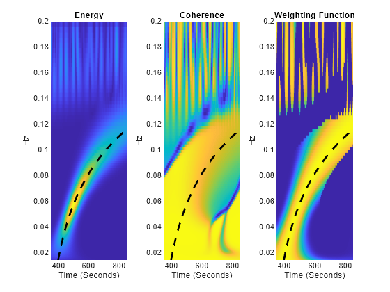
Calculate the theoretical group velocity for both the reference and perturbed waveforms. Select a time region of interest in the seismograms of [350,850] seconds. Plot the theoretical group velocity over this interval along with the magnitude of the wavelet cross spectrum, coherence, and weighting function to demonstrate that the high-magnitude areas of the wavelet cross spectrum and cross-spectrum based weighting function provide an approximation to the group velocity dispersion.

diffCref = -1.6.*omega-0.87;
uref= cref.^2./(cref-diffCref.*omega);
diffCcurr = -2*omega-1;
ucurr = ccurr.^2./(ccurr-diffCcurr.*omega);
uAvg = mean([uref(:) ucurr(:)],2);
groupvel = dist./uAvg;
tlim = [350 850];
tiledlayout(1,3)
nexttile
hp = pcolor(t,freq,abs(wcs));
hp.EdgeColor = "none";
xlabel("Time (Seconds)")
ylabel("Hz")
hold on
plot(groupvel,f,"k--",LineWidth=2)
hold off
title("Energy")
xlim(tlim)
nexttile
hp = pcolor(t,freq,wcoh);
hp.EdgeColor = "none";
xlabel("Time (Seconds)")
ylabel("Hz")
hold on
plot(groupvel,f,"k--",LineWidth=2)
hold off
xlim(tlim)
title("Coherence")
nexttile
hp = pcolor(t,freq,weights);
hp.EdgeColor = "none";
xlabel("Time (Seconds)")
ylabel("Hz")
hold on
plot(groupvel,f,"k--",LineWidth=2)
hold off
title("Weighting Function")
xlim(tlim)

Figure contains 3 axes objects. Axes object 1 with title Energy, xlabel Time (Seconds), ylabel Hz contains 2 objects of type surface, line. Axes object 2 with title Coherence, xlabel Time (Seconds), ylabel Hz contains 2 objects of type surface, line. Axes object 3 with title Weighting Function, xlabel Time (Seconds), ylabel Hz contains 2 objects of type surface, line.

Unwrap the phase in the cross spectrum and plot the unwrapped phase along with group velocity in the area of the time-frequency plane with high coherence.

xwt = wcs;
tIdx = find(t>= tlim(1) & t<= tlim(2));
fIdx = find(freq >=.02 & freq <= 0.1);
lowcoherence = find(weights(fIdx,tIdx) < coherenceThresh);
phasexwt = angle(xwt(fIdx,tIdx));
phasexwt(lowcoherence) = NaN;
phaseUnwrapXWT = unwrap(phasexwt,[],2);
figure
hp = pcolor(t(tIdx),freq(fIdx),phaseUnwrapXWT);
hp.EdgeColor = "none";
c = colorbar;
c.Label.String = "Phase (rad)";
hold on
plot(dist./uAvg,f,"k--",LineWidth=2)
clim([-2,8])
xlabel('Time (Seconds)')
ylabel('Frequency (Hz)')
set(gca,'fontsize',12)
ht = title("Unwrapped Around Group Velocity");
ht.FontSize = 13;
hold off

Figure contains an axes object. The axes object with title Unwrapped Around Group Velocity, xlabel Time (Seconds), ylabel Frequency (Hz) contains 2 objects of type surface, line.

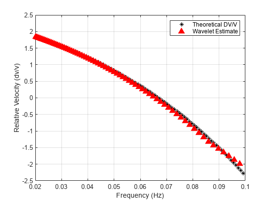
Calculate the theoretical relative velocity (dv/v) and compare against the result obtained using the wavelet cross spectrum.

tref = dist./cref;
tcurr = dist./ccurr;
Drefcurr = (tcurr-tref)';
tdmean = mean([tref(:),tcurr(:)],2);
dofT = -Drefcurr./tdmean;
dtUnwrapWeighted = phaseUnwrapXWT./(2*pi*freq(fIdx));
meandt = mean(dtUnwrapWeighted,2,"omitnan");
Td = 1./f;
tcd = spline(f,tdmean,freq(fIdx));
dv_unwrapped = -meandt./tcd;
h1 = plot(f,dofT*100,"k*");
hold on
h2 = plot(freq(fIdx),dv_unwrapped*100,"r^", ...
    MarkerSize=8,MarkerFaceColor=[1 0 0]);
xlim([0.02 0.1]); ylim([-2.5,2.5])
grid on
xlabel("Frequency (Hz)")
ylabel("Relative Velocity (dv/v)")
legend("Theoretical DV/V","Wavelet Estimate")
hold off

Figure contains an axes object. The axes object with xlabel Frequency (Hz), ylabel Relative Velocity (dv/v) contains 2 objects of type line. One or more of the lines displays its values using only markers These objects represent Theoretical DV/V, Wavelet Estimate.

Note that the wavelet estimates provide a good fit to the theoretical relative velocity changes.

Relative Velocity from Coda-Wave Simulations

The following section illustrates the application of wavelet cross spectral analysis on synthetic coda waveforms. The details of the simulation are provided in section 3.1 of Mao et al. (2020). The authors have kindly permitted the use of the simulated data in this example. The simulated model is contained the file synthetic_dvov_0.05percent.mat (Copyright (c) 2019, Shujuan Mao and Aurélien Mordret, covered by MIT License). The file dt-wavelet.rights is a text file included in the example folder and contains the licensing for this data. You can consult this license information if you wish by entering:

>>edit dt-wavelet.rights

at the MATLAB command prompt.

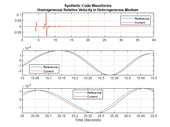
The key parameter for the following is that the authors generated the current model by linearly increasing the velocity in the reference model by 0.05 percent. This means that the relative velocity is a constant 0.05. Load the data and plot the coda waveforms. The data are sampled at 500 Hz and simulated for 40 seconds. Zoom in on portions of the waveforms over intervals of [15,15.5] and [25,25.5] seconds to show the phase relationships more clearly.

% Copyright (c) 2019, Shujuan Mao and Aurélien Mordret, covered by MIT License.
load("synthetic_dvov_0.05percent.mat")
origWave = ori_waveform';
currWave = new_waveform';
tiledlayout(3,1)
nexttile
plot(time, [origWave currWave])
grid on
axis tight
legend("Reference","Current")
xlim([0,40])
title({"Synthetic Coda Waveforms" ; ...
    "Homogeneous Relative Velocity in Heterogeneous Medium"})
nexttile
plot(time, [origWave currWave])
grid on
axis tight
legend("Reference","Current")
xlim([15,15.5])
legend("Reference","Current",Location="best")
nexttile
plot(time, [origWave currWave])
grid on
axis tight
xlabel("Time (Seconds)")
xlim([25,25.5])
legend("Reference","Current",Location="best")

Obtain the wavelet coherence and cross spectra using frequency limits from 0.5 to 5 Hz and 16 voices per octave. Smooth the coherence and cross spectrum estimates over three scales. In this case, base the estimates on the smoothed wavelet cross spectrum.

[wcoh,wcs,freq,coi,wtori,wtcurr] = wcoherence(origWave,currWave,Fs, ...
    FrequencyLimits=[0.5 5],VoicesPerOctave=16,NumScalesToSmooth=3);

Calculate the weighting function based on equation 12 in Mao et al., (2020) using the global maximum of the phase. Because the two waveforms are essentially perfectly coherent, utilize a high threshold of 0.95 for the coherence. Plot the cross-spectrum weighting function.

thresh = 0.95;
weights = weightedxwt(wcoh,wcs,thresh,MaxMethod="global");

Obtain bandlimited measures of the time delays estimated from the weighted wavelet cross spectrum. Use the following four octave bands, [0.5,1.0], [0.75,1.5], [1.0,2.0], and [1.5,3.0] Hz.

Use a 20-second window of the reference and current waveforms from 15 to 35 seconds. The helper function localXWTmeasures included at the end of the example returns these estimates.

freqbands = [0.5,1.0; 0.75,1.5; 1.0,2.0; 1.5,3.0];
timelimits = [15,35];
[dtmatrix,dtotvec,dtotfvec,timewindow] = ...
    localXWTmeasures(wcs,weights,time,freq,timelimits,freqbands);

Plot the local time-delay measurements along with the least-squares fits and the expected model in each octave band.

tiledlayout(4,1)
for ii = 1:4
    nexttile
    plot(timewindow, -dtmatrix(ii,:),"*-")
    hold on
    plot(time, -dtotvec(ii).*time,"-",LineWidth=1.25)
    plot(time, 0.05.*time./100,"--",LineWidth=1.0)
    hold off
    axis tight
    grid on    
    ylabel("\Deltat (s)")
    title("Frequency Band "+ ...
        num2str(freqbands(ii,1))+"-"+num2str(freqbands(ii,2))+" Hz")  
end
xlabel("Travel time (Seconds)")
legend("\Deltat measured with wavelet","Best fitting line","Model", ...
    location="bestoutside")

$Figure contains 4 axes objects. Axes object 1 with title Frequency Band 0.5-1 Hz, ylabel \Deltat (s) contains 3 objects of type line. Axes object 2 with title Frequency Band 0.75-1.5 Hz, ylabel \Deltat (s) contains 3 objects of type line. Axes object 3 with title Frequency Band 1-2 Hz, ylabel \Deltat (s) contains 3 objects of type line. Axes object 4 with title Frequency Band 1.5-3 Hz, xlabel Travel time (Seconds), ylabel \Deltat (s) contains 3 objects of type line. These objects represent \Deltat measured with wavelet, Best fitting line, Model.$

Note the wavelet estimates demonstrate excellent agreement with the model across all the octave bands.

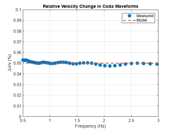
Finally, plot the relative velocity measurements as a function of frequency obtained using the wavelet method. Recall the model here should be a constant 0.05.

figure
plot(freq,-dtotfvec.*100,"*",MarkerSize=9,LineWidth=2.0)
hold on
plot(freq, ones(size(freq)).*0.05,"--",LineWidth=2.0)
hold off
legend("Measured","Model")
axis tight
grid on
xlabel("Frequency (Hz)")
ylabel("\Deltav/v (%)")
ylim([0,0.1])
xlim([0.5,3])
title("Relative Velocity Change in Coda Waveforms")

Figure contains an axes object. The axes object with title Relative Velocity Change in Coda Waveforms, xlabel Frequency (Hz), ylabel Delta v/v blank (%) contains 2 objects of type line. One or more of the lines displays its values using only markers These objects represent Measured, Model.

The wavelet method again provides very good agreement with the theoretical model over the frequency range of interest.

Summary

This example demonstrates the ability of wavelet coherence and the wavelet cross spectrum to obtain high-quality estimates of the dispersive velocity changes in seismic waveforms. While this example concentrated on seismic applications, the ability of wavelet coherence and the associated cross spectrum to characterize frequency-dependent phase (time) relationships between two signals in the time-frequency plane makes it applicable to and useful for nonstationary signals in general.

References

Shujuan Mao, Aurelien Mordret, Michel Campillo, Hongjian Fang, Robert D van der Hilst, "On the measurement of seismic traveltime changes in the time–frequency domain with wavelet cross-spectrum analysis", Geophysical Journal International, Volume 221, Issue 1, April 2020, Pages 550–568, https://doi.org/10.1093/gji/ggz495.

Appendix

function weights = weightedxwt(wcoh,xwt,thresh,NVargs)
% This function is only intended for the example
% Algorithm due to Mao et al., 2020
arguments
    wcoh
    xwt
    thresh
    NVargs.MaxMethod {mustBeTextScalar,...
        mustBeMember(NVargs.MaxMethod,["time","global"])} = "time"
end
logXWT = log(1+abs(xwt));
if startsWith(NVargs.MaxMethod,'t')
    freqWeights = max(log(1+abs(xwt)),[],2);
else
    freqWeights = repmat(max(log(abs(xwt)),[],'all'), ...
        size(xwt,1),size(xwt,2));
end
weights = logXWT./freqWeights;
if startsWith(NVargs.MaxMethod,'g')
    weights = weights+1;
end
weights(wcoh < thresh) = 0;
end

function [dtmatrix,dtotvec,dtotfvec,timewindow] = ...
    localXWTmeasures(wcs,weights,time,freq,timelimits,freqbands)
dt_xy = unwrap(angle(wcs))./(2*pi*freq);
timeIdx = find(time>=timelimits(1) & time<=timelimits(2));
timewindow = time(timeIdx);
numfreqbands = size(freqbands, 1);
dtotvec = zeros(numfreqbands,1);
dtmatrix = zeros(numfreqbands,numel(timeIdx));
for ii = 1:numfreqbands
    dt_vec_iband = zeros(numel(timeIdx),1);
    ifreq_band = freqbands(ii,:);
    ifre_ind = find((freq>=ifreq_band(1)) & (freq<=ifreq_band(2)));
    ifre = freq(ifre_ind);
    angle_mat_iband = unwrap(angle(wcs(ifre_ind,timeIdx)));    
    for jj = 1:numel(timeIdx)
        j_time_ind = timeIdx(jj);
        weighted_dt = lscov(2*pi*ifre,angle_mat_iband(:,jj), ...
            weights(ifre_ind,j_time_ind));        
        dt_vec_iband(jj) = weighted_dt;
    end    
    dtmatrix(ii,:) = dt_vec_iband;
    dtotvec(ii) = lscov(timewindow',dt_vec_iband);    
    dtotfvec = zeros(size(freq));
    for kk = 1:length(dtotfvec)
        idtot = lscov(timewindow',dt_xy(kk,timeIdx)', ...
            (weights(kk,timeIdx))');
        dtotfvec(kk) = idtot; 
    end
end
end