Detect Anomalies in ECG Data Using Wavelet Scattering and LSTM Autoencoder in Simulink

Data Description

This example uses ECG data obtained from the Sudden Cardiac Death Holter Database [1]. This database contains a collection of long-term ECG recordings of patients who experienced sudden cardiac death during the recordings. The dataset includes data from patients who sustained different types of ventricular tachyarrhythmia such as atrial fibrillation, ventricular tachycardia etc.

This example uses ECG data from only one of the patients with a history of ventricular tachycardia and attempts to detect anomalies in the ECG data of the patient caused by ventricular tachycardia. The ECG signal has a sampling rate of 250 Hz.

Download and Prepare Data

Download the data from https://ssd.mathworks.com/supportfiles/SPT/data/PhysionetSDDB.zip using the downloadSupportFile function. The data set contains 320 seconds of ECG data of the patient and the downloaded file contains two timetables. The timetable X contains the ECG signal of the patient. Timetable Y contains the annotated labels that indicate whether each sample of the ECG signal is normal. You use the labels only to visualize the dataset.

datasetZipFile = matlab.internal.examples.downloadSupportFile('SPT','data/PhysionetSDDB.zip');
dataFolder = fullfile(tempdir,'PhysionetSDDB');
unzip(datasetZipFile,dataFolder);
ds2 = load(fullfile(dataFolder,"sddb49.mat"));
ecgSignals = ds2.X;
ecgLabels = ds2.y;

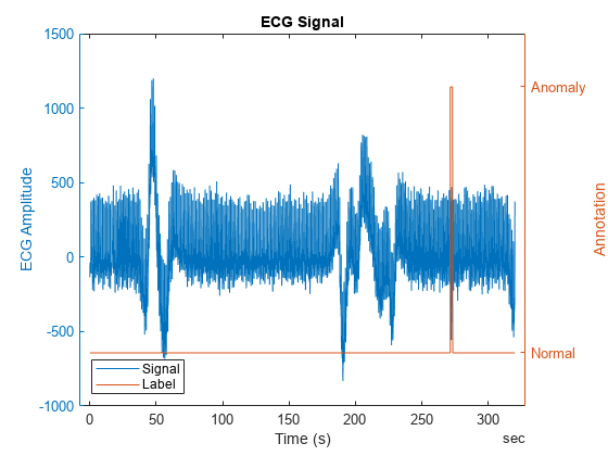
Visualize the ECG data by overlaying the annotated anomalies. Zoom in on the plot to observe the region of the anomaly better.

Notice that the ECG data contains gradual changes in the baseline of the ECG signal. These gradual changes are known as baseline drifts. Baseline drifts are caused by factors such as respiration, movement artifacts, changes in skin impedance etc and happens often in normal ECG data as well. Anomaly detection in ECG signals is challenging because these changes in baseline level can be misclassified as anomalies.

figure;
yyaxis left
plot(ecgSignals.Time,ecgSignals.Variables);
title("ECG Signal");
ylabel("ECG Amplitude")
yyaxis right;
plot(ecgSignals.Time,ecgLabels.anomaly)
xlabel("Time (s)")
legend(["Signal" "Label"],Location="southwest");
ylabel("Annotation")
yticks([0 1]);yticklabels({'Normal','Anomaly'})
ylim([-0.2,1.2]);

Split the data set into training and testing sets. A common approach to choosing training data is to use a segment of the signal where it is evident that there are no anomalies. In many situations, the beginning of a recording is usually normal, such as in this ECG signal. Choose the first 200 seconds of the recording to train the model with purely normal data. Use the rest of the recording to test the performance of the anomaly detector. The training data contains segments with baseline drift. Ideally, the detector learns and adapts to the baseline drift and considers it normal.

fs = 250;
idxTrain = 1:200*fs;
idxTest = idxTrain(end)+1:height(ecgSignals);
dataTrain = ecgSignals(idxTrain,:);
dataTest = ecgSignals(idxTest,:);

Normalize the training data using the normalize function and obtain the mean and standard deviation from the output arguments C and S respectively. We will use this value of mean and standard deviation to normalize the input data in Simulink when running the model.

[dataProcessedTrain,C,S] = normalize(dataTrain);
meanVal = C.DISTORTEDsddb49

meanVal = 
-30.4565

stdVal = S.DISTORTEDsddb49

stdVal = 
197.2967

Wavelet Scattering Network

Wavelet scattering is a powerful tool for signal analysis that captures both low-frequency and high-frequency information. An input signal is convolved with a series of wavelet filters at multiple scales and positions, and the resulting coefficients are passed through nonlinearities and averaging to produce low-variance representations of time series. This process enables the extraction of robust and discriminative features insensitive to shifts in the input signal. For more information on feature extraction using wavelet scattering, see Wavelet Scattering (Wavelet Toolbox).

By decomposing the ECG signal into different frequency bands using wavelet transforms, wavelet scattering can effectively separate the baseline drift from the underlying cardiac activity. The wavelet scattering coefficients provide a representation of the signal that is more robust to baseline drift while remaining sensitive to other anomalies in the signal. By extracting features from these coefficients, it becomes possible to analyze the ECG signal while mitigating the effects of baseline drift.

In this example, you partition the sequences into smaller regions, each with a duration of 1 second, and assign a single detection label to each region. Split the 200 seconds long training data into 200 sequences of length 1 second. Use an invariance scale of 1 sec. To have a sufficient number of scattering coefficients per time window to average, set OversamplingFactor to 4 to produce a sixteen-fold increase in the number of scattering coefficients for each path with respect to the critically downsampled value. With these settings, you obtain 200 scattering paths with 63 scattering coefficients for each path.

N = 250; 
sn = waveletScattering(SignalLength=N,SamplingFrequency=fs,...
    InvarianceScale=1,OversamplingFactor=4);

[spaths,npaths] = paths(sn);
npaths=sum(npaths)

npaths = 
200

ncoeffs = numCoefficients(sn)

ncoeffs = 
63

Exclude the zeroth-order scattering coefficients and convert the features to cell arrays. To improve the robustness of the features to baseline drift and better detect higher frequency anomalies, consider removing additional lower-order coefficients.

Xtrain = reshape(dataProcessedTrain.DISTORTEDsddb49,N,[]);
trainfeat = featureMatrix(sn,Xtrain);
trainfeat = trainfeat(2:end,:,:);
trainfeatcell = squeeze(num2cell(trainfeat,[2,1]));

LSTM Autoencoder

Autoencoders are used to detect anomalies in a signal. The autoencoder is trained on features extracted from data without anomalies. As a result, the learned network weights minimize the reconstruction error for features extracted from ECG data without anomalies. The statistics of the reconstruction error for the training data can be used to select the threshold in the anomaly detection block that determines the detection performance of the autoencoder. The detection block declares the presence of an anomaly when it encounters a reconstruction error above threshold. This example uses a deepSignalAnomalyDetectorLSTM object to create the LSTM autoencoder-based anomaly detector.

Create the anomaly detector object using the deepSignalAnomalyDetector function. The network has one LSTM layer in the Encoder with 64 hidden units and one LSTM layer in the Decoder with 64 hidden units. Note that we can use a smaller network here with one layer each in the encoder and decoder because the extracted features are robust and insensitive to baseline drifts. Set the number of input channels to npaths–1 since the zeroth-order coefficients are excluded. Set the WindowLength to 'fullSignal' since we need a single label of anomaly detection for the feature matrix corresponding to each second of input data.

detector = deepSignalAnomalyDetector(npaths-1,"lstmautoencoder",...
    EncoderHiddenUnits=64,DecoderHiddenUnits=64,WindowLength='fullSignal');

Specify the hyperparameters. Use Adam optimization and a mini-batch size of 50. Set the maximum number of epochs to 50.

options = trainingOptions('adam',...
    SequenceLength=ncoeffs,...
    MaxEpochs=50,...
    MiniBatchSize=50,...
    Plots='training-progress',...
    Verbose=false);

Train the detector.

trainDetector(detector,trainfeatcell,options);

Adjust Threshold and Save the Detector Model

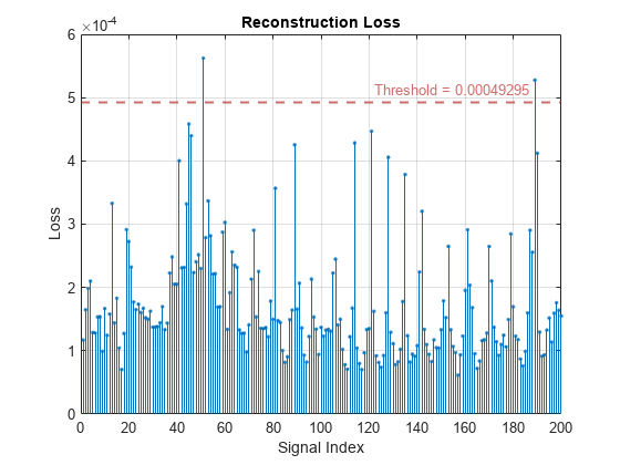
The statistics of reconstruction error computed using the training data can be used to determine the threshold which is to be used for detecting anomalies in the ECG data during inference. Compute the RMSE between the input features and reconstructed features of the training data.

figure; plotLoss(detector,trainfeatcell);

Increase the threshold value to 6e-4 since the input data is known to not contain any anomalies.

threshold = 6e-4;
updateDetector(detector,ThresholdMethod = 'manual',Threshold = threshold);

Save the detector model and parameters to a MAT file using the saveModel method. The generated MAT-file will be used by the Deep Signal Anomaly Detector block to load the trained network and detector parameters for realtime detection.

saveModel(detector,'trainedDetectorECG.mat');

Open the Simulink model

Open the attached Simulink model. Use this model to extract wavelet scattering features and detect anomalies in ECG data using a network that has been trained using the steps mentioned in this example.

open_system('ECGAnomalyDetection.slx');

Warning: Unrecognized function or variable 'CloneDetectionUI.internal.CloneDetectionPerspective.register'.

Read the test ECG data at 250 samples per second into frames of duration 1 second, i.e, 250 samples each. Normalize the data using Normalize subsystem block by providing the mean and standard deviation values calculated from the training data on the dialog box. Pass the normalized ECG data to the Wavelet Scattering block. Use the same parameters which were used to extract features from the training data to configure the Wavelet Scattering block. Provide the extracted features to the Deep Signal Anomaly Detector block. The Deep Signal Anomaly Detector block requires DSP Systems Toolbox™ and Deep Learning Toolbox™ licenses.

Set the Detector MAT-file path parameter of the Deep Signal Anomaly Detector block to trainedDetectorECG.mat, which is the MAT-file generated in the previous step, that contains the trained network and anomaly detection parameters. The Deep Signal Anomaly Detector block passes the input through the trained network to reconstruct the input signal and thresholds the loss between input and reconstructed signals to detect anomalies. You can set the Parameters for post-processing to "Read from MAT-file" to read the parameters from the MAT-file, or you can set it to "Specify on dialog" to specify the values of the parameters individually. In this example, set the Parameters for post-processing to "Specify on dialog". Set Window length value to ncoeff which is 63 and Overlap length to 0, since we need a single label of anomaly detection for the feature matrix corresponding to each second of input data. Set threshold to 6e-4 which is the value we determined in the earlier section.

The Delay output of the Deep Signal Anomaly Detector block calculates the delay added to the input signal by the block in terms of number of samples. Use a Delay block to delay the input signal by number of samples equal to the calculated delay value to align the input signal with the Anomaly and Window loss outputs.

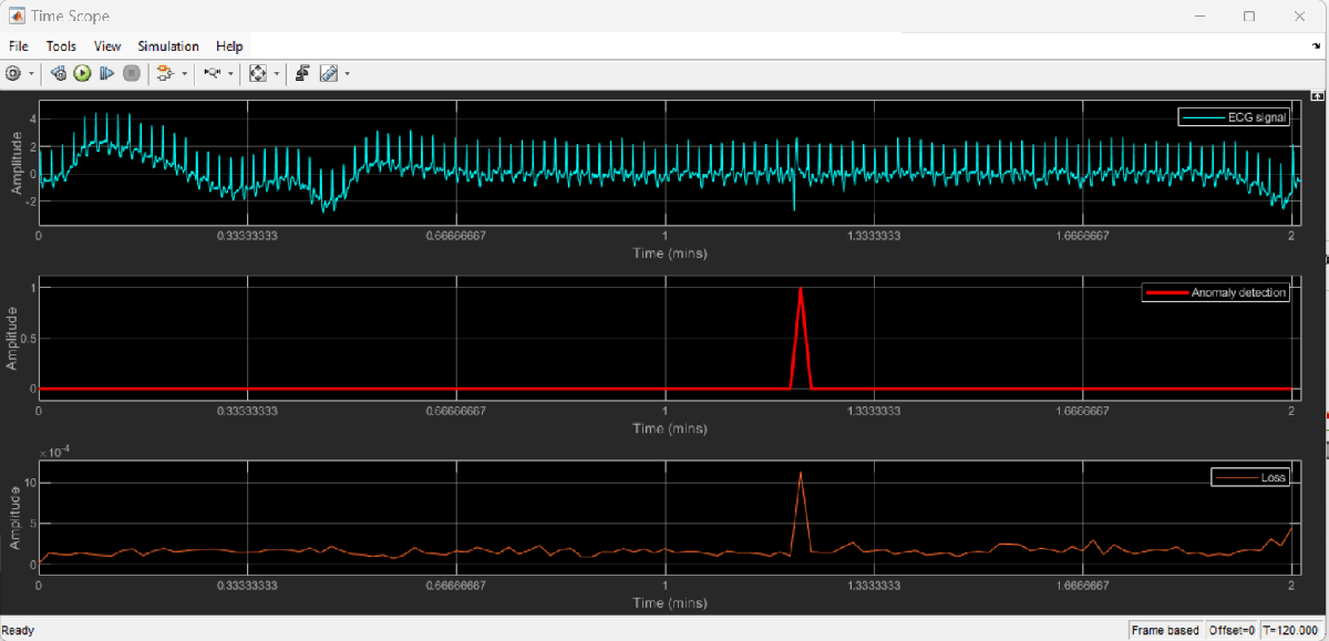
Visualize the delayed signal, anomaly flag and window loss using Time Scope.

Simulate the model.

sim('ECGAnomalyDetection.slx');

On the Time Scope, observe the ECG signal and the logical decision of anomaly detection. The portion of input signal corresponding to a decision of 0 represents normal signal and the portion of signal corresponding to a decision of 1 represents anomalous region. Each data point in the anomaly detection signal corresponds to a one-second region of the input signal.

Analysis

Extract features from the test data.

dataProcessedTest = normalize(dataTest,"center",C,"scale",S);
Xtest = reshape(dataProcessedTest.DISTORTEDsddb49,N,[]);
testfeat = featureMatrix(sn,Xtest);
testfeat = testfeat(2:end,:,:);
testfeatcell = squeeze(num2cell(testfeat,[2,1]));

Compute the reconstruction loss between input and reconstructed features for training and test data.

[~,lossTest] = detect(detector,testfeatcell);
[~,lossTrain] = detect(detector,trainfeatcell);
lossTest = [lossTest{:}]; % convert cell array to vector
lossTrain = [lossTrain{:}];% convert cell array to vector

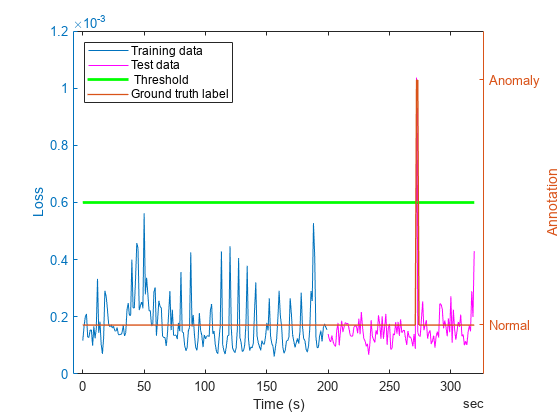
Plot the threshold value and loss values for the train data, test data, and overlay the annotation labels on the plot.

Observe from the low loss values that the network manages to reconstruct the data well. For region of the data containing anomalies, the network gives an error which is significantly higher than the error for normal signal, thereby helping in robust detection of anomalies. Notice that the regions corresponding to baseline drifts in the signal have relatively higher loss compared to other regions. However, this loss value is significantly less compared to the loss value in the regions where anomalies are seen.

figure;
yyaxis left;
plot(dataTrain.Time(1:N:end),lossTrain);
hold on;
plot(dataTest.Time(1:N:end),lossTest,'m-');
plot(ecgSignals.Time(1:N:end),threshold*ones(height(ecgSignals.Time(1:N:end)),1),'g-',LineWidth=2);
xlabel('Time (s)');
ylabel ('Loss');
yyaxis right
plot(ecgSignals.Time(1:N:end),ecgLabels.anomaly(1:N:end),LineWidth=1);
yticks([0 1]);yticklabels({'Normal','Anomaly'})
ylim([-0.2,1.2]);
ylabel("Annotation")
legend(["Training data" "Test data" " Threshold" "Ground truth label"],Location="northwest");

References

[1] Greenwald, Scott David. "Development and analysis of a ventricular fibrillation detector." (M.S. thesis, MIT Dept. of Electrical Engineering and Computer Science, 1986).
[2] Nawaz M, Ahmed J (2022) Cloud-based healthcare framework for real-time anomaly detection and classification of 1-D ECG signals. PLoS ONE 17(12): e0279305. https://doi.org/10.1371/journal.pone.0279305
See Also
deepSignalAnomalyDetectorLSTM | Wavelet Scattering | Repeat | Time Scope
Topics
- Wavelet Scattering (Wavelet Toolbox)
- Detect Air Compressor Sounds in Simulink Using Wavelet Scattering
- Detect Anomalies in Machinery Using LSTM Autoencoder
- Real-Time Noise Detection on Raspberry Pi Using Deep Signal Anomaly Detector
- Fault Detection Using Wavelet Scattering and Recurrent Deep Networks (Wavelet Toolbox)
- Real-Time ECG QRS Detection