Digit Classification with Wavelet Scattering

Digit Images

The dataset used in this example contains 10,000 synthetic images of digits from 0 to 9. The images are generated by applying random transformations to images of those digits created with different fonts. Each digit image is 28-by-28 pixels. The dataset contains an equal number of images per category. Use the imageDataStore to read the images.

digitDatasetPath = fullfile(matlabroot,'toolbox','nnet','nndemos','nndatasets','DigitDataset');
Imds = imageDatastore(digitDatasetPath,'IncludeSubfolders',true, 'LabelSource','foldernames');

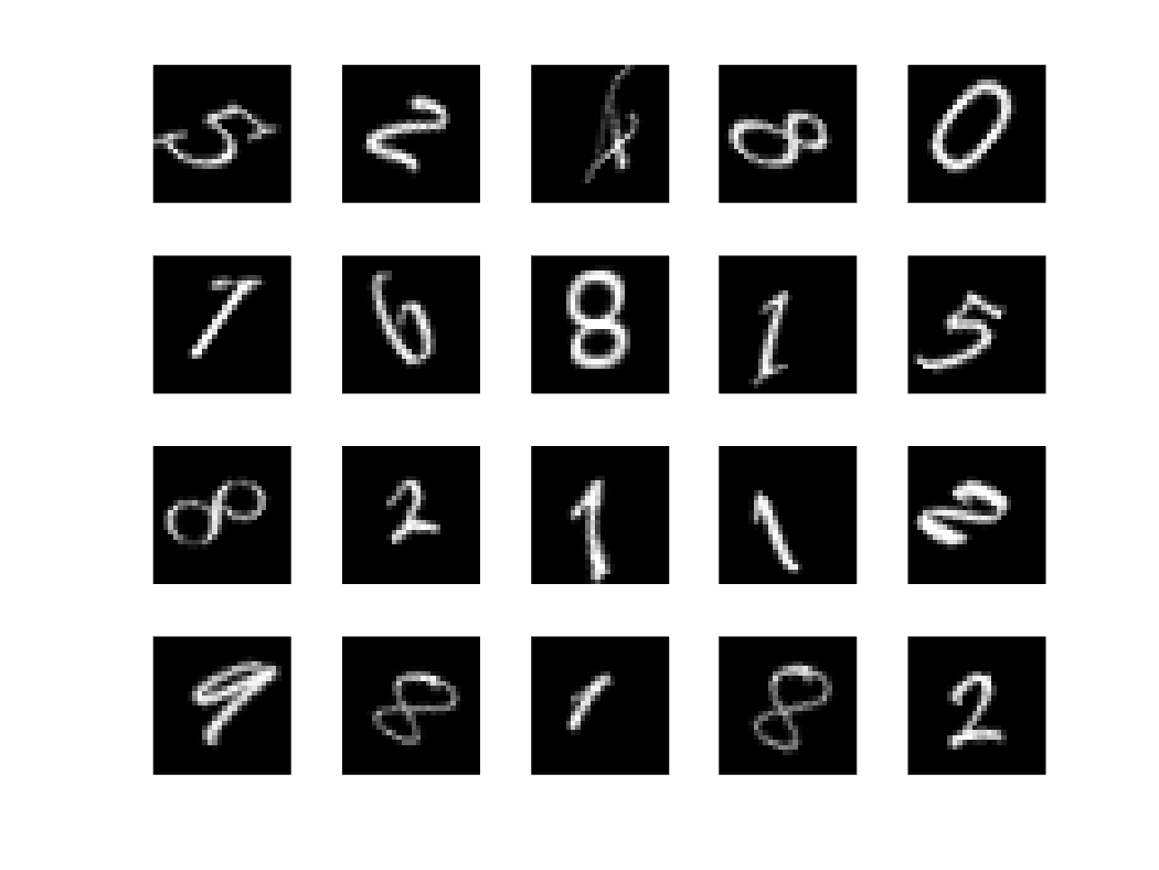
Randomly select and plot 20 images from the dataset.

figure
numImages = 10000;
rng(100);
perm = randperm(numImages,20);
for np = 1:20
    subplot(4,5,np);
    imshow(Imds.Files{perm(np)});
end

You can see that the 8s exhibit considerable variability while all being identifiable as an 8. The same is true of the other repeated digits in the sample. This is consistent with natural handwriting where any digit differs non-trivially between individuals and even within the same individual's handwriting with respect to translation, rotation, and other small deformations. Using wavelet scattering, we hope to build representations of these digits which obscure this irrelevant variability.

Wavelet Image Scattering Feature Extraction

The synthetic images are 28-by-28. Create a wavelet image scattering framework and set the invariance scale to equal the size of the image. Set the number of rotations to 8 in each of the two wavelet scattering filter banks. The construction of the wavelet scattering framework requires that we set only two hyperparameters: the InvarianceScale and NumRotations.

sf = waveletScattering2('ImageSize',[28 28],'InvarianceScale',28, ...
    'NumRotations',[8 8]);

This example uses MATLAB®'s parallel processing capability through the tall array interface. If a parallel pool is not currently running, you can start one by executing the following code. Alternatively, the first time you create a tall array, the parallel pool is created.

if isempty(gcp)
    parpool;
end

Starting parallel pool (parpool) using the 'LocalProfile1' profile ...
14-Nov-2023 14:19:36: Job Queued. Waiting for parallel pool job with ID 1 to start ...
Connected to parallel pool with 6 workers.

For reproducibility, set the random number generator. Shuffle the files of the imageDatastore and split the 10,000 images into two sets, one for training and one held-out set for testing. Allocate 80% of the data, or 8,000 images, to the training set and hold out the remaining 2,000 images for testing. Create tall arrays from the training and test datasets. Use the helper function helperScatImages to create feature vectors from the scattering transform coefficients. helperScatImages obtains the log of the scattering transform feature matrix as well as the mean along both the row and column dimensions of each image. The code for helperScatImages is at the end of this example. For each image in this example, the helper function creates a 217-by-1 feature vector.

rng(10);
Imds = shuffle(Imds);
[trainImds,testImds] = splitEachLabel(Imds,0.8);
Ttrain = tall(trainImds);
Ttest = tall(testImds);
trainfeatures = cellfun(@(x)helperScatImages(sf,x),Ttrain,'UniformOutput',false);
testfeatures = cellfun(@(x)helperScatImages(sf,x),Ttest,'UniformOutput',false);

Use tall's gather capability to concatenate all the training and test features.

Trainf = gather(trainfeatures);

Evaluating tall expression using the Parallel Pool 'LocalProfile1':
- Pass 1 of 1: Completed in 2 min 48 sec
Evaluation completed in 2 min 48 sec

trainfeatures = cat(2,Trainf{:});
Testf = gather(testfeatures);

Evaluating tall expression using the Parallel Pool 'LocalProfile1':
- Pass 1 of 1: Completed in 38 sec
Evaluation completed in 38 sec

testfeatures = cat(2,Testf{:});

The previous code results in two matrices with row dimensions 217 and column dimension equal to the number of images in the training and test sets respectively. Accordingly, each column is a feature vector for its corresponding image. The original images contained 784 elements. The scattering coefficients represent an approximate 4-fold reduction in the size of each image.

PCA Model and Prediction

This example constructs a simple classifier based on the principal components of the scattering feature vectors for each class. The classifier is implemented in the functions helperPCAModel and helperPCAClassifier. helperPCAModel determines the principal components for each digit class based on the scattering features. The code for helperPCAModel is at the end of this example. helperPCAClassifier classifies the held-out test data by finding the closest match (best projection) between the principal components of each test feature vector with the training set and assigning the class accordingly. The code for helperPCAClassifier is at the end of this example.

model = helperPCAModel(trainfeatures,30,trainImds.Labels);
predlabels = helperPCAClassifier(testfeatures,model);

After constructing the model and classifying the test set, determine the accuracy of the test set classification.

accuracy = sum(testImds.Labels == predlabels)./numel(testImds.Labels)*100

accuracy = 
  99.599999999999994

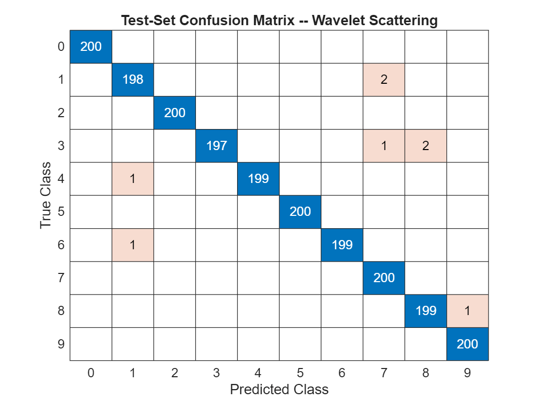
We have achieved 99.6% correct classification of the test data. To see how the 2,000 test images have been classified, plot the confusion matrix. There are 200 examples in the test set for each of the 10 classes.

figure;
confusionchart(testImds.Labels,predlabels)
title('Test-Set Confusion Matrix -- Wavelet Scattering')

CNN

In this section, we train a simple convolutional neural network (CNN) to recognize digits. Construct the CNN to consist of a convolution layer with 20 5-by-5 filters with 1-by-1 strides. Follow the convolution layer with a RELU activation and max pooling layer. Use a fully connected layer, followed by a softmax layer to normalize the output of the fully connected layer to probabilities.

imageSize = [28 28 1];
layers = [ ...
    imageInputLayer([28 28 1])
    convolution2dLayer(5,20)
    reluLayer
    maxPooling2dLayer(2,'Stride',2)
    fullyConnectedLayer(10)
    softmaxLayer
    ];

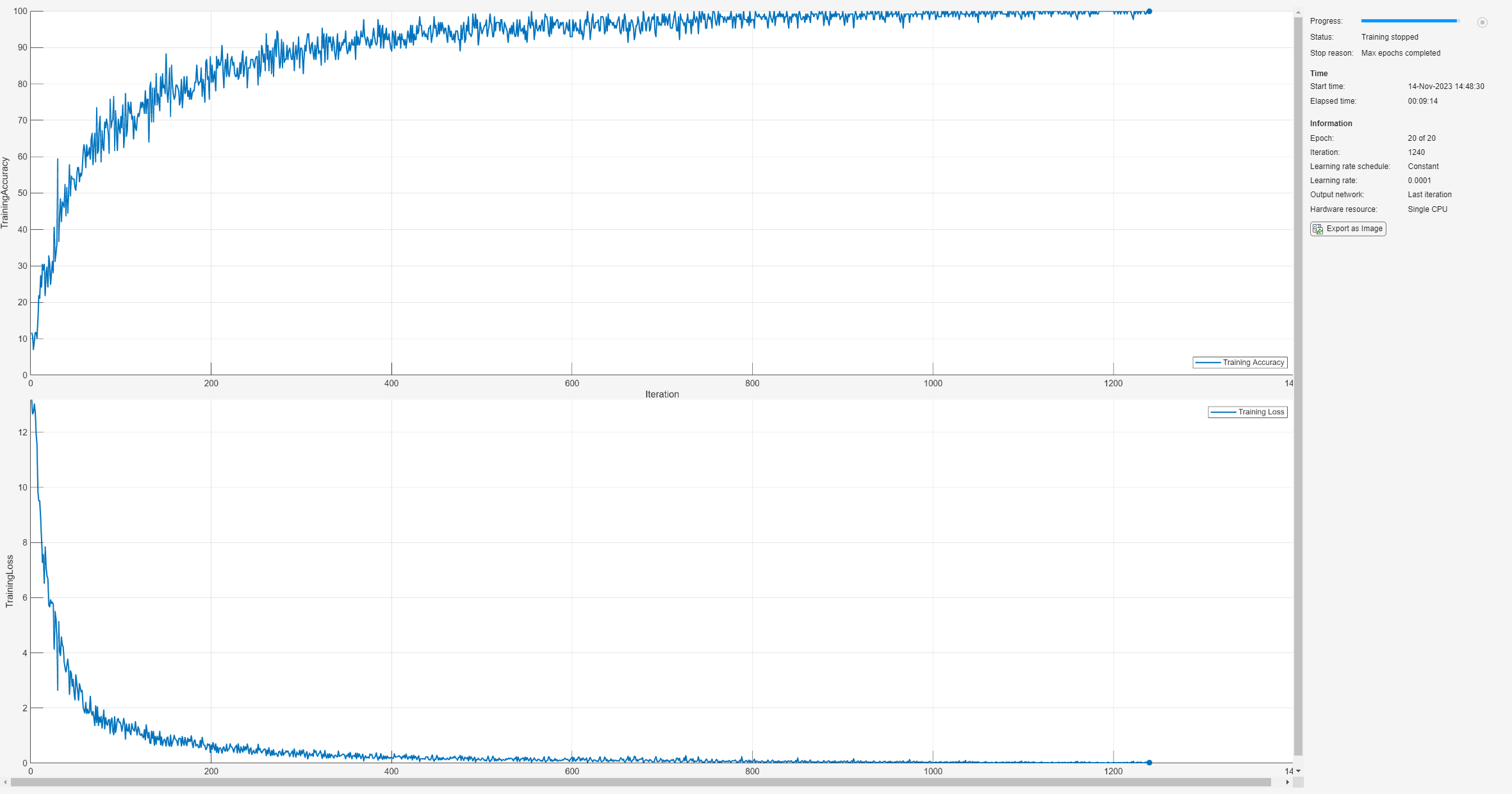
Specify the training options. Use stochastic gradient descent with momentum and a learning rate of 0.0001 for training. Set the maximum number of epochs to 20. Display the training progress in a plot and monitor the accuracy. For reproducibility, set the ExecutionEnvironment to 'cpu'.

options = trainingOptions('sgdm', ...
    'MaxEpochs',20,...
    'InitialLearnRate',1e-4, ...
    'Verbose',false, ...
    'Plots','training-progress', ...
    'Metrics','accuracy', ...
    'ExecutionEnvironment','cpu');

Train the neural network using the trainnet (Deep Learning Toolbox) function. For classification, use cross-entropy loss. By default, the trainnet function uses a GPU if one is available. Training on a GPU requires a Parallel Computing Toolbox™ license and a supported GPU device. For information on supported devices, see GPU Computing Requirements (Parallel Computing Toolbox). Otherwise, the trainnet function uses the CPU. To specify the execution environment, use the ExecutionEnvironment training option.

For training and testing we use the same data sets used in the scattering transform.

reset(trainImds);
reset(testImds);
net = trainnet(trainImds,layers,"crossentropy",options);

By the end of training, the CNN is performing near 100% on the training set. Use the trained network to make predictions on the held-out test set.

classNames = categories(trainImds.Labels);
scores = minibatchpredict(net,testImds,'ExecutionEnvironment','cpu');
YPred = scores2label(scores,classNames);
DCNNaccuracy = sum(YPred == testImds.Labels)/numel(YPred)*100

DCNNaccuracy = 
  94.450000000000003

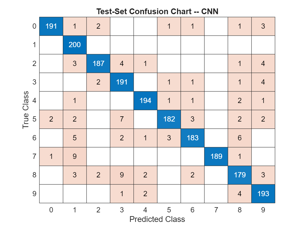
The simple CNN has achieved around 95% correct classification on the held-out test set. Plot the confusion chart for the CNN.

figure;
confusionchart(testImds.Labels,YPred)
title('Test-Set Confusion Chart -- CNN')

Summary

This example used wavelet image scattering to create low-variance representations of digit images for classification. Using the scattering transform with fixed filter weights and a simple principal components classifier, we achieved 99.6% correct classification on a held-out test set. With a simple CNN in which the filters are learned, we achieved around 95% correct. This example is not intended as a direct comparison of the scattering transform and CNNs. There are multiple hyperparameter and architectural changes you can make in each case, which significantly affect the results. The goal of this example was simply to demonstrate the potential of deep feature extractors like the wavelet scattering transform to produce robust representations of data for learning.

References

[1] Bruna, J., and S. Mallat. "Invariant Scattering Convolution Networks." IEEE Transactions on Pattern Analysis and Machine Intelligence. Vol. 35, Number 8, 2013, pp. 1872–1886.

[2] Mallat, S. "Group Invariant Scattering." Communications in Pure and Applied Mathematics. Vol. 65, Number 10, 2012, pp. 1331–1398.

[3] Sifre, L., and S. Mallat. "Rotation, scaling and deformation invariant scattering for texture discrimination." 2013 IEEE Conference on Computer Vision and Pattern Recognition. 2013, pp 1233–1240. 10.1109/CVPR.2013.163.

Appendix — Supporting Functions

helperScatImages

function features = helperScatImages(sf,x)
% This function is only to support examples in the Wavelet Toolbox.
% It may change or be removed in a future release.

% Copyright 2018 MathWorks

smat = featureMatrix(sf,x,'transform','log');
features = mean(mean(smat,2),3);
end

helperPCAModel

function model = helperPCAModel(features,M,Labels)
% This function is only to support wavelet image scattering examples in 
% Wavelet Toolbox. It may change or be removed in a future release.
% model = helperPCAModel(features,M,Labels)

% Copyright 2018 MathWorks

% Initialize structure array to hold the affine model
model = struct('Dim',[],'mu',[],'U',[],'Labels',categorical([]),'s',[]);
model.Dim = M;
% Obtain the number of classes
LabelCategories = categories(Labels);
Nclasses = numel(categories(Labels));
for kk = 1:Nclasses
    Class = LabelCategories{kk};
    % Find indices corresponding to each class
    idxClass = Labels == Class;
    % Extract feature vectors for each class
    tmpFeatures = features(:,idxClass);
    % Determine the mean for each class
    model.mu{kk} = mean(tmpFeatures,2);
    [model.U{kk},model.S{kk}] = scatPCA(tmpFeatures);
    if size(model.U{kk},2) > M
        model.U{kk} = model.U{kk}(:,1:M);
        model.S{kk} = model.S{kk}(1:M);
        
    end
    model.Labels(kk) = Class;
end
    
function [u,s,v] = scatPCA(x,M)
	% Calculate the principal components of x along the second dimension.

	if nargin > 1 && M > 0
		% If M is non-zero, calculate the first M principal components.
	    [u,s,v] = svds(x-sig_mean(x),M);
	    s = abs(diag(s)/sqrt(size(x,2)-1)).^2;
	else
		% Otherwise, calculate all the principal components.
        % Each row is an observation, i.e. the number of scattering paths
        % Each column is a class observation
		[u,d] = eig(cov(x'));
		[s,ind] = sort(diag(d),'descend');
		u = u(:,ind);
	end
end
end

helperPCAClassifier

function labels = helperPCAClassifier(features,model)
% This function is only to support wavelet image scattering examples in 
% Wavelet Toolbox. It may change or be removed in a future release.
% model is a structure array with fields, M, mu, v, and Labels
% features is the matrix of test data which is Ns-by-L, Ns is the number of
% scattering paths and L is the number of test examples. Each column of
% features is a test example.

% Copyright 2018 MathWorks

labelIdx = determineClass(features,model); 
labels = model.Labels(labelIdx); 
% Returns as column vector to agree with imageDatastore Labels
labels = labels(:);


%--------------------------------------------------------------------------
function labelIdx = determineClass(features,model)
% Determine number of classes
Nclasses = numel(model.Labels);
% Initialize error matrix
errMatrix = Inf(Nclasses,size(features,2));
for nc = 1:Nclasses
    % class centroid
    mu = model.mu{nc};
    u = model.U{nc};
    % 1-by-L
    errMatrix(nc,:) = projectionError(features,mu,u);
end
% Determine minimum along class dimension
[~,labelIdx] = min(errMatrix,[],1);   


%--------------------------------------------------------------------------
function totalerr = projectionError(features,mu,u)
    %
    Npc = size(u,2);
    L = size(features,2);
    % Subtract class mean: Ns-by-L minus Ns-by-1
    s = features-mu;
    % 1-by-L
    normSqX = sum(abs(s).^2,1)';
    err = Inf(Npc+1,L);
	err(1,:) = normSqX;
    err(2:end,:) = -abs(u'*s).^2;
    % 1-by-L
    totalerr = sqrt(sum(err,1));
end
end
end