Acoustic Scene Classification with Wavelet Scattering

Data

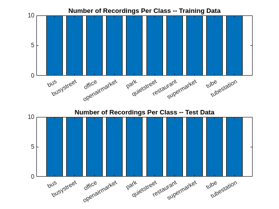
The training and test sets used in this example are taken from the Detection and Classification of Acoustic Scenes and Events (DCASE) 2013 challenge [3]. The training data consist of 100 waveforms recorded in 10 different environments: bus, busy street, office, open-air market, park, quiet street, restaurant, supermarket, tube (subway), and tube station (subway station) [1]. There are 10 recordings per environment in the training set. The test set consists of an additional 10 recordings in each of the previous environments. Each two-channel recording is 30 seconds long sampled at 44.1 kHz. This results in 1323000 samples per recording. See [1] for additional details on the data.

Download the DCASE 2013 challenge data set, DCASE2013.zip, file from the MathWorks website, https://ssd.mathworks.com/supportfiles/WA/data/DCASE2013.zip. The data is saved under userpath. See the help for userpath if you wish to change this destination. After downloading and unzipping, the data set folder contains a text file, license.txt, with the required licensing information and attributions for the DCASE 2013 challenge data. Additionally, there are two subfolders, scenes_stereo and scenes_stereo_testset. Those folders contain the .wav files for the training and test sets, respectively. The unzipped data requires about 977 MB of disk space.

datasetZipFile = matlab.internal.examples.downloadSupportFile('WA','data/DCASE2013.zip');
datasetFolder = fullfile(fileparts(datasetZipFile),'DCASE2013');
if ~exist(datasetFolder,'dir')     
    unzip(datasetZipFile,datasetFolder);
end

Use an audioDatastore to manage data access. Set up the audioDatastore to read the training data. Extract the environment labels from the filenames.

trainlabels = filenames2labels(fullfile(datasetFolder,"scenes_stereo"),ExtractBefore=digitsPattern);
adsTrain = audioDatastore(fullfile(datasetFolder,"scenes_stereo"),OutputDataType="single");
adsTrain.Labels = trainlabels;

Follow the same procedure for the test data.

testlabels = filenames2labels(fullfile(datasetFolder,"scenes_stereo_testset"),ExtractBefore=digitsPattern);
adsTest = audioDatastore(fullfile(datasetFolder,"scenes_stereo_testset"),OutputDataType="single");
adsTest.Labels = testlabels;

Examine the number of recordings in each category for the training and test data.

tiledlayout(2,1)
nexttile
bar(unique(trainlabels),countcats(trainlabels))
title("Number of Recordings Per Class -- Training Data")
nexttile
bar(unique(testlabels),countcats(testlabels))
title("Number of Recordings Per Class -- Test Data")

In the hierarchy of machine learning problems, acoustic scene classification is one of the most challenging. Judging a scene based on acoustic cues alone is difficult because many scenes share similar characteristics. Note the obvious similarity between some of the environments included in this data. These include the similarity between tube and tubestation, openairmarket and busystreet just to cite a couple examples. Top performance on these DCASE challenges often does not exceed 80%. In this particular challenge the top performance was 76% on the test set [3]. You can find the overall rankings and test performance by scene for this contest at the following site: https://dcase.community/challenge2013/task-acoustic-scene-classification-results.

Time and Joint Time-Frequency Scattering Features

Wavelet scattering transforms are signal representations built with wavelet multiscale decompositions in a deep convolutional framework [2]. The convolutional part of the framework comes from the wavelet transform, while pointwise modulus operations serve as the nonlinear activation. Pooling is achieved by simple averaging, or lowpass filtering. Scattering representations often provide both dimensionality reduction and robust features for machine learning applications. For a brief introduction to scattering representations and additional references see Wavelet Scattering. This example uses both time scattering and joint time-frequency scattering representations. Time-frequency scattering supplements time scattering with additional convolutions and averaging across frequency.

Time and Time-Frequency Scattering Networks

Set up the time and time-frequency scattering networks used in this example. For the time scattering network, set the invariance scale to one second of data. At a sample rate of 44.1 kHz, that results in 44100 samples. Use the default number of filter banks and the default quality factors of 8 wavelets per octave in the first filter bank and 1 wavelet per octave in the second filter bank. To reduce the computational complexity of the problem, use the central 262144 (2^18) samples of the data, or 5.94 seconds of the 30 second recording.

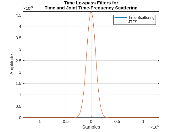
tsn = waveletScattering(SignalLength=262144,InvarianceScale=44100,Precision="single");

In the time scattering network, the invariance scale of 44100 samples corresponds to $$\pm 2.5758\sigma$$ for the Gaussian lowpass filter, where $$\sigma$$ is the time standard deviation. In timeFrequencyScattering, this corresponds to a TimeInvarianceScale of 6992 samples determined by the following code. See the documentation on joint time-frequency scattering for details.

basesigma = 0.13;
T = round((2*pi*basesigma)/(2*2.5758)*44100);

Construct a JTFS network. For now, focus only on signal length and time invariance scale, T. Obtain the lowpass filters used in the time scattering and JTFS networks and demonstrate their equivalence.

jtfsn = timeFrequencyScattering(SignalLength=262144,TimeQualityFactors=8, ...
    TimeInvarianceScale=T,FrequencyInvarianceScale=4,FrequencyQualityFactor=2, ...
    NumTimeOctaves=9,NumFrequencyOctaves=4,TimeMaxPaddingFactor=0, ... 
    FrequencyMaxPaddingFactor=1,FilterDataType="single");
[~,~,phifJTFS] = filterbank(jtfsn);
filters = filterbank(tsn);
phifTS = filters{1}.phift;
phitJTFS = ifftshift(ifft(phifJTFS));
phitTS = ifftshift(ifft(phifTS));
t = -2^17:2^17-1;
figure
plot(t,[phitTS phitJTFS])
xlabel("Samples")
ylabel("Amplitude")
grid on
axis tight
title(["Time Lowpass Filters for"; ...
    "Time and Joint Time-Frequency Scattering"])
legend("Time Scattering","JTFS")

In this example, identical parameters for both networks are used in the specification of the time and JTFS networks where possible. For the JTFS parameters with no equivalence in time scattering, use 9 octaves for both time filter banks and 4 octaves for the frequency filter bank. Specify the FrequencyInvarianceScale to be 4 quefrencies. See the JTFS documentation for details on JTFS parameters.

Time Scattering and Joint Time-Frequency Scattering Features

To obtain the time scattering and JTFS features, define transforms which trim each audio signal to 262144 (2^18) samples, compute the mean across the two channels, and return the time scattering and JTFS transforms. For the JTFS transform, the transform function, jtfsFeatures, excludes the "SpinUp" and "U2JointLowPass" coefficients.

jtfsTransformTrain = transform(adsTrain,@(x)jtfsFeatures(x,jtfsn));
jtfsTransformTest = transform(adsTest,@(x)jtfsFeatures(x,jtfsn));
tsTransformTrain = transform(adsTrain,@(x)tsFeatures(x,tsn));
tsTransformTest = transform(adsTest,@(x)tsFeatures(x,tsn));

Using the datastore readall function, compute all the features for the training and test sets. If you have Parallel Computing Toolbox™, accelerate the computation using a parallel pool. If you do not have Parallel Computing Toolbox™, set UseParallelPool to false. Using a parallel pool, the feature extraction takes around 8 minutes.

UseParallelPool = true;
currP = gcp("nocreate");
if UseParallelPool && isempty(currP)
    parpool(3);
end

Starting parallel pool (parpool) using the 'Processes' profile ...
Connected to parallel pool with 3 workers.

jtfsFeaturesTrain = readall(jtfsTransformTrain,UseParallel=UseParallelPool);
jtfsFeaturesTest = readall(jtfsTransformTrain,UseParallel=UseParallelPool);
tsFeaturesTrain = readall(tsTransformTrain,UseParallel=UseParallelPool);
tsFeaturesTest = readall(tsTransformTest,UseParallel=UseParallelPool);

Reshape the JTFS features for use in machine learning models. There is no need to reshape the time scattering features.

numExamples = 100;
numJTFSpaths = size(jtfsFeaturesTrain,1)/numExamples;
numJTFSFreq = size(jtfsFeaturesTrain,2);
numJTFSTime = size(jtfsFeaturesTrain,3);
jtfsFeaturesTrain = reshape(jtfsFeaturesTrain,numJTFSpaths,100,numJTFSFreq,numJTFSTime);
jtfsFeaturesTest = reshape(jtfsFeaturesTest,numJTFSpaths,100,numJTFSFreq,numJTFSTime);
jtfsFeaturesTrain = permute(jtfsFeaturesTrain,[4 2 3 1]);
jtfsFeaturesTest = permute(jtfsFeaturesTest,[4 2 3 1]);
jtfsFeaturesTrain = reshape(jtfsFeaturesTrain,numJTFSTime*100,...
        numJTFSFreq*numJTFSpaths);
jtfsFeaturesTest = reshape(jtfsFeaturesTest,numJTFSTime*100,...
        numJTFSFreq*numJTFSpaths);

Training Machine Learning Models

In this section, we train support vector machines (SVM) on the scattering features. Set up and fit the SVM. Use a cubic polynomial kernel and set the BoxConstraint to 999 and OutlierFraction to 0.1 to guard against overfitting in the one-vs-one coding scheme. Set up the SVM template.

classNames = unique(trainlabels);
rng default
templateJTFS = templateSVM(...
    KernelFunction = "polynomial", ...
    PolynomialOrder=3, ...
    KernelScale="auto", ...
    BoxConstraint=999, ...
    Standardize=true, ...
    OutlierFraction=0.1);

Fit the SVM to the training data.

svmJTFS = fitcecoc(...
    jtfsFeaturesTrain, ...
    repelem(trainlabels,numJTFSTime), ...
    Learners=templateJTFS, ...
    Coding="onevsone", ...
    ClassNames=classNames);

Apply the trained model to the test set. Use a majority vote on the 64 time windows of the JTFS transform. If there is no unique mode based on the 64 JTFS time windows, the prediction is labeled an error.

predLabelsJTFS = predict(svmJTFS,jtfsFeaturesTest);
[ClassVotesTestJTFS,ClassCountsTestJTFS]  = helperMajorityVoteAS(predLabelsJTFS,...
testlabels,unique(testlabels));
sum(ClassVotesTestJTFS == testlabels)/numExamples*100 %#ok<*NOPTS>

ans = 
100

Repeat the same procedure for time scattering features.

numTSTime = size(tsFeaturesTrain,1)/100;
templateTS = templateSVM(...
    KernelFunction = "polynomial", ...
    PolynomialOrder=3, ...
    KernelScale="auto", ...
    BoxConstraint=999, ...
    Standardize=true, ...
    OutlierFraction=0.1);

svmTS = fitcecoc(...
    tsFeaturesTrain, ...
    repelem(trainlabels,numTSTime), ...
    Learners=templateTS, ...
    Coding="onevsone", ...
    ClassNames=classNames);

Apply the trained model to the test set. Use a majority vote on the 32 time windows of the time scattering transform. Similar to JTFS, if there is no unique mode, the prediction is labeled an error.

predLabelsTS = predict(svmTS,tsFeaturesTest);
[ClassVotesTestTS,ClassCountsTestTS]  = helperMajorityVoteAS(predLabelsTS,...
testlabels,unique(testlabels));
sum(ClassVotesTestTS == testlabels)/numExamples*100

ans = 
78

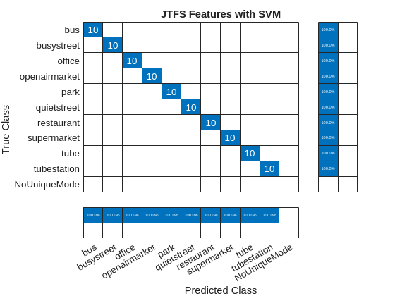
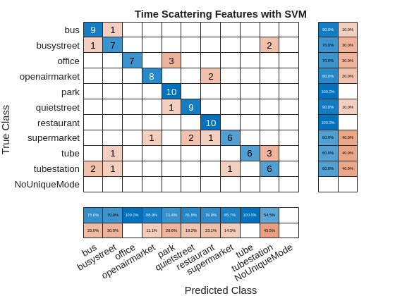
The performance for the JTFS features on the test set with an SVM is excellent. The model trained with the time scattering features does not perform as well as the JTFS features, but is on the level of the best performance shown at DCASE 2013: https://dcase.community/challenge2013/task-acoustic-scene-classification-results. Plot the corresponding confusion charts for the two methods.

figure
confusionchart(testlabels,ClassVotesTestJTFS,...
    RowSummary="row-normalized",ColumnSummary="column-normalized",...
    Title= "JTFS Features with SVM");

figure
confusionchart(testlabels,ClassVotesTestTS,...
    RowSummary="row-normalized",ColumnSummary="column-normalized",...
    Title="Time Scattering Features with SVM");

Summary

SVMs were trained on the DCASE 2013 Challenge [3] data using time and joint time-frequency scattering representations. Both scattering representations provided robust features for machine learning as demonstrated by their performance on this challenging task. However, the additional frequency invariance provided by JTFS achieved superior results to time scattering. JTFS performance on the test data is approximately 100%, while time scattering achieves approximately 78%, which is still a couple percentage points above the highest result achieved in the contest. Efforts were made to ensure that the time and JTFS networks were as similar as possible. However, it is certainly possible that different hyperparameters could improve the performance of time scattering.

References

Dimitrios Giannoulis, Dan Stowell, Emmanouil Benetos, Mathias Rossignol, Mathieu Lagrange, and Mark. D. Plumbley. "A database and challenge for acoustic scene classification and event detection." In 21st European Signal Processing Conference (EUSIPCO 2013), 1–5. Sep. 2013.

Mallat, Stephane. “Group Invariant Scattering.” Communications on Pure and Applied Mathematics 65, no. 10 (July 24, 2012): 1331–98. https://doi.org/10.1002/cpa.21413.

Stowell, Dan, Dimitrios Giannoulis, Emmanouil Benetos, Mathieu Lagrange, and Mark D. Plumbley. “Detection and Classification of Acoustic Scenes and Events.” IEEE Transactions on Multimedia 17, no. 10 (October 2015): 1733–46. https://doi.org/10.1109/tmm.2015.2428998.

Appendix

The following helper functions are used in this example.

function smat = jtfsFeatures(audio,jtfsn)
data = mean(audio,2);
data = trimdata(data,2^18,Side="both");
smat = scatteringFeatures(jtfsn,data,...
    ExcludeCoefficients=["SpinUp","U2JointLowpass"]);
end

function smat = tsFeatures(audio,tsn)
data = mean(audio,2);
data = trimdata(data,2^18,Side="both");
smat = featureMatrix(tsn,data);
smat = smat';
end