Share Results

Step 5 of 5 in Using Wavelet Signal Analyzer App

Export Analyses

You can export all decompositions and compressed signals from Wavelet Signal Analyzer to the workspace. First select a decomposition in Scenarios. The app displays the decomposition names in the Scenario pane in the format scenarioName.

To export the decomposition of the original signal, click Export ▼. Under Decomposition Coefficients, select To Workspace. The app creates the workspace variable scenarioNameDecomposition in the workspace.
To export the decomposition of the compressed signal, click Export ▼. Under Compressed Signal, select Coefficients to Workspace. The app creates the workspace variable scenarioNameCompressedCoefficients in the workspace.
To export the compressed signal, click Export ▼. Under Compressed Signal, select To Workspace. The app creates the workspace variable scenarioNameCompressed in the workspace.

In all cases, text in the status bar confirms the export. If the variable already exists in the workspace, Wavelet Signal Analyzer gives you the option to cancel the export. You can then rename either the scenario or the variable. Otherwise, the app overwrites the existing variable.

Generate Scripts

You can generate scripts to recreate all decompositions and compressed signals in your workspace. First select a decomposition in Scenarios.

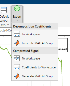
To recreate the decomposition of the original signal, click Export ▼. Under Decomposition Coefficients, select Generate MATLAB Script.
To recreate the compression workflow, click Export ▼. Under Compressed Signal, select Generate MATLAB Script.

In both cases, an untitled script opens in your editor with executable code. You can then save the script.

Example: Compress Signal and Generate Script

Open Live Script

This example shows how to compress a signal and generate a script to recreate the compressed signal in the workspace.

Import Data

Load the electrical consumption signal.

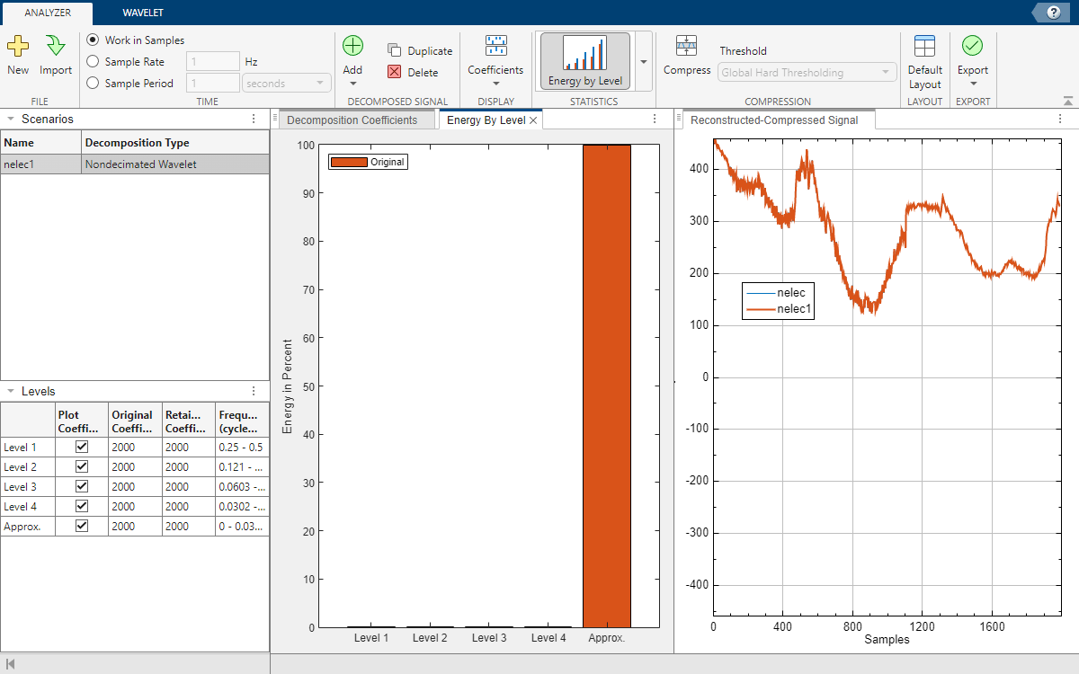
load nelec

Open Wavelet Signal Analyzer and import the signal into the app. By default, a four-level nondecimated wavelet decomposition of the signal appears. The table in the Levels pane indicates that there are 2000 original and retained coefficients at all levels. Plot the relative energies of the decomposition. Most of the energy lies in the approximation coefficients.

Compress Signal

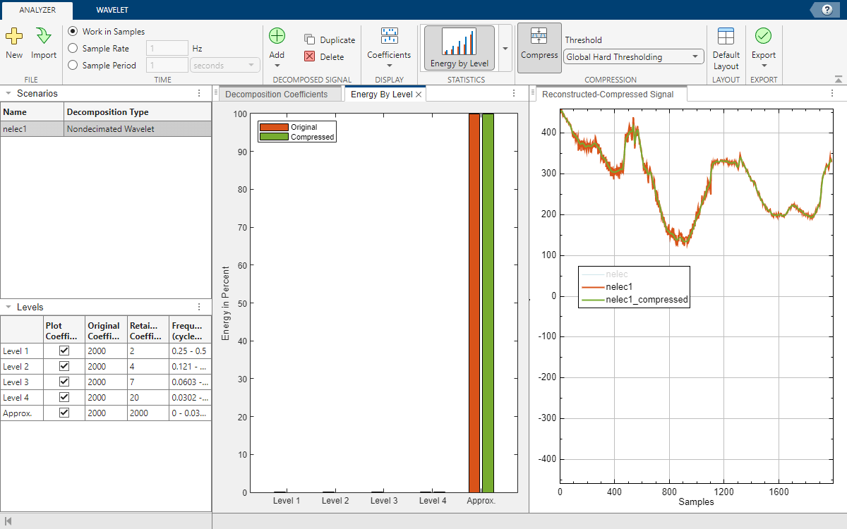
On the Analyzer tab, click Compress. The app applies the same default threshold thr to the coefficients using global hard thresholding. The app sets all coefficients that lie in the interval [–thr, thr] to 0.

The Levels pane reports the number of coefficients retained at each level after thresholding.
The Energy By Level pane updates to include the retained coefficients.
The Reconstructed-Compressed Signal pane now includes a plot of the compressed signal, nelec1_compressed. Click nelec and nelec1 in the plot legend to show only the compressed signal.

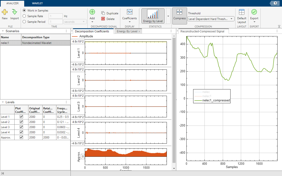
wavelet-signal-analyzer-generate-script-1.5.png

Switch to the Decomposition Coefficients pane. Compress the signal. Set 0 to all the detail coefficients. Use all the approximation coefficients to construct the compressed signal.

In any level coefficients plot, drag the horizontal cursor to the maximum threshold. The number of retained coefficients in the entire decomposition is 0.
Switch to level dependent hard thresholding. Then in the approximation coefficients plot, enter 0 in the text field to retain all the approximation coefficients.

Generate Script

You have a number of export options available. You can export the original coefficients or generate a script to recreate the decomposition in your workspace. Because you have enabled compression, you can also export the compressed signal or thresholded coefficients, as well as generate a script to recreate the compressed signal in your workspace. To recreate the compressed signal in your workspace, in the Export ▼ menu, select Generate MATLAB Script under Compressed Signal.

An untitled script opens in your editor with the following executable code. You can save the script as is or modify it to apply the same compression to other signals. Run the code.

Note: The app uses time-aligned coefficients only when visualizing the decomposition. The generated script always uses the original coefficients. The state of the Time Align parameter has no impact on the generated script.

% Perform the decomposition using MODWT
numberOfLevels = 4;
wt = modwt(nelec,"sym4",numberOfLevels);

% Compute the energy by level for the decomposition
energyByLevel = 100*sum((wt.^2),2)/sum(wt.^2,"all");

% Thresholds for compressing the imported signal
compressionThresholds = ...
    [464.1 464.1 464.1 464.1 0]';

% Duplicate coefficients for thresholding
wc = wt;

% Apply threshold to coefficients
for idx = 1:numel(compressionThresholds)
    thr = abs(compressionThresholds(idx));
    w = wc(idx,:);
    w = wthresh(w,"h",thr);
    wc(idx,:) = w;
end

% Energy by level for the compressed signal
energyByLevelForCompressed = 100*sum((wc.^2),2)/sum(wc.^2,"all");

% Reconstruct the compressed signal using IMODWT
nelec1_compressed = imodwt(wc,"sym4");

Plot the original signal, nelec, and the compressed signal, nelec1_compressed.

plot(nelec)
hold on
plot(nelec1_compressed,LineWidth=2)
hold off
axis tight
title("Original and Compressed Signals")
legend("Original","Compressed")

Figure contains an axes object. The axes object with title Original and Compressed Signals contains 2 objects of type line. These objects represent Original, Compressed.

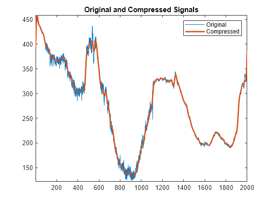
Compare the energies by level of the original and thresholded coefficients. Because you set all the wavelet (detail) coefficients to 0, all the energy in the thresholded coefficients is contained in the approximation level.

[energyByLevel energyByLevelForCompressed]

ans = 5×2

    0.0152         0
    0.0124         0
    0.0125         0
    0.0260         0
   99.9338  100.0000

Workflow

Previous Step	Current Step
Compress Signal	Share Results

Share Results

Export Analyses

Generate Scripts

Example: Compress Signal and Generate Script

Workflow

See Also

Apps

Related Topics