Signal Deconvolution and Impulse Denoising Using Pursuit Methods

Open Live Script

We show two examples of sparse recovery algorithms. The first example shows how to use orthogonal matching pursuit to recover ground profile information from noisy seismic signal measurements. In the second example, we show how basis pursuit can be used to remove impulse noise from power system current measurements.

Pursuit methods are popular recovery methods, which attempt to find sparse representations of signals in overcomplete dictionaries. Orthogonal matching pursuit is a class of iterative algorithms that chooses dictionary elements in a greedy manner that best approximates the signal. In contrast, basis pursuit tries to find the best approximation of the signal with respect to the dictionary such that the recovered signal has a minimum $ℓ_{1}$ norm.

Example 1: Sparse Seismic Deconvolution With Orthogonal Matching Pursuit

Sparse seismic deconvolution is one of the oldest inverse problems in the field of seismic imaging [1]. The sparse seismic deconvolution process aims to recover the structure of ocean-bottom sediments from noisy seismic signals. The ocean bottom is modeled as a sparse signal x with a few impulses that correspond to the interfaces between layers in the ground. The observed noisy seismic signal y is modeled as

$y = D x + w,$

where

D is the convolution operator and the columns of the operator correspond to a wavelet filter $h (t) = (1 - \frac{t^{2}}{s^{2}}) \exp (- \frac{t^{2}}{2 s^{2}})$ .
The vector w is the observation noise.

Since the convolution suppresses many low and high frequencies, we need some prior information to regularize the inverse problem. The sparse seismic deconvolution process employs pursuit algorithms to recover the sparse signal x. In the first part of this example, we demonstrate how matching pursuit can be used to recover a sparse impulse signal from a seismic observation vector.

Generate Seismic Filter

The sparse signal, wavelet, and dictionary used in this example are generated following the steps in [2].

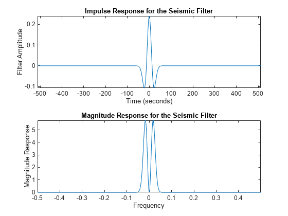
Generate a seismic filter h, which is denoted by the second derivative of a Gaussian.

n = 1024;
s = 13;
% Generate the seismic filter
t = -n/2:n/2-1;
h = (1-t.^2/s^2).*exp( -(t.^2)/(2*s^2) );
h = h-mean(h);
h = h/norm(h);
% Frequency response for the seismic filter
h1 = fftshift(h);
hf = fftshift(abs(fft(h1)));
f = t/n;

Display the impulse response and frequency response of the seismic filter.

tiledlayout(2,1)
nexttile
plot(t,h)
title("Impulse Response for the Seismic Filter")
xlabel("Time (seconds)")
ylabel("Filter Amplitude")
axis tight
nexttile
plot(f,hf)
title("Magnitude Response for the Seismic Filter")
xlabel("Frequency")
ylabel("Magnitude Response")
axis tight

Figure contains 2 axes objects. Axes object 1 with title Impulse Response for the Seismic Filter, xlabel Time (seconds), ylabel Filter Amplitude contains an object of type line. Axes object 2 with title Magnitude Response for the Seismic Filter, xlabel Frequency, ylabel Magnitude Response contains an object of type line.

Generate the deconvolution operator matrix D that will be used for orthogonal matching pursuit. To stabilize the recovery, we downsample the impulse response by a factor of 2.

% Build the deconvolution operator matrix D
[Y,X] = meshgrid(1:2:n,1:n);
D = reshape( h1(mod(X-Y,n)+1), [n n/2]);

Observe the columns of the deconvolution operator.

figure
imagesc(D)
colormap("bone")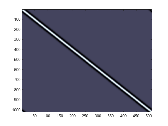

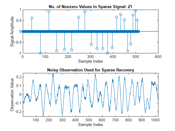
Figure contains an axes object. The axes object contains an object of type image.

Create the sparse signal x using random amplitudes and signs for the impulses. Next, generate the noisy observations y by first multiplying the sparse signal x with the deconvolution operator matrix D and adding noise to the product.

% Generate the sparse signal
x = sparseSignal(n/2);
% Obtain noisy observations
sigma = .06*max(h);
w = randn(n,1)*sigma;
y = D*x + w;

Plot the sparse signal and the corresponding noisy observation vector.

tiledlayout(2,1)
nexttile
strng = strcat("No. of Nonzero Values in Sparse Signal: ",num2str(nnz(x)));
stem(x)
title(strng)
xlabel("Sample Index")
ylabel("Signal Amplitude")
nexttile
plot(y)
axis tight
title("Noisy Observation Used for Sparse Recovery")
xlabel("Sample Index")
ylabel("Observation Value")

Figure contains 2 axes objects. Axes object 1 with title No. of Nonzero Values in Sparse Signal: 21, xlabel Sample Index, ylabel Signal Amplitude contains an object of type stem. Axes object 2 with title Noisy Observation Used for Sparse Recovery, xlabel Sample Index, ylabel Observation Value contains an object of type line.

Sparse Spike Deconvolution With Orthogonal Matching Pursuit

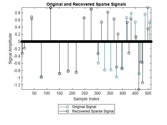
Use orthogonal matching pursuit to recover the sparse signal. Orthogonal matching pursuit is a greedy algorithm that has been popularly employed for sparse signal recovery. The algorithm greedily picks the column of the dictionary that is orthogonal to the current residual. The indices of the identified atoms correspond to the nonzero entries in the sparse signal to be recovered.

We perform the deconvolution process using the following steps.

Generate the sensing dictionary that corresponds to the convolution operator matrix D.

A = sensingDictionary(CustomDictionary=D);

Use orthogonal matching pursuit to deconvolve the noisy observation vector y. Plot the recovered sparse signal.

% Use matching pursuit to recover the sparse signal
[Xr, YI, ~, ~] = matchingPursuit(A,y,Algorithm="OMP");
figure
stem(x) 
hold on
stem(Xr,"k")
hold off
axis tight
title("Original and Recovered Sparse Signals")
legend("Original Signal","Recovered Sparse Signal",Location="southoutside")
xlabel("Sample Index")
ylabel("Signal Amplitude")

Figure contains an axes object. The axes object with title Original and Recovered Sparse Signals, xlabel Sample Index, ylabel Signal Amplitude contains 2 objects of type stem. These objects represent Original Signal, Recovered Sparse Signal.

Plot the best fit to the noisy signal.

plot(y) 
hold on
plot(YI,"k")
hold off
axis tight
title({"Observed Noisy Measurement and"; "Best Fit Recovered From Orthogonal Matching Pursuit"})
legend("Observed Noisy Measurement","Best Orthogonal Matching Pursuit Fit",Location="southoutside")
xlabel("Sample index")
ylabel("Signal amplitude")

Figure contains an axes object. The axes object with title Observed Noisy Measurement and Best Fit Recovered From Orthogonal Matching Pursuit, xlabel Sample index, ylabel Signal amplitude contains 2 objects of type line. These objects represent Observed Noisy Measurement, Best Orthogonal Matching Pursuit Fit.

Summary

In this example, we demonstrated how the ocean bottom structure can be recovered from a noisy seismic observation signal using an orthogonal matching pursuit algorithm. The recovery process exploited the knowledge that the seismic signal is sparse with respect to the wavelet basis. The deconvolution process enables researchers to understand more about the structure of ocean bottom given the seismic signal reflected from it.

Example 2: Impulse Denoising in Line Current Using Basis Pursuit

This section shows how to denoise power line signals using basis pursuit. In power line communications (PLC) networks, the electrical distribution grid is used as a data transmission medium for reduced cost and expenditure. Impulse noise in PLC networks is a significant problem as it can corrupt the data sent by the receiver. This type of corruption arises from the connection and disconnection of electrical devices, operation of circuit breaks and isolators in the power network, etc.

The problem at hand is to denoise current measurements by separating the current signal from the impulse noise. To do this we find a representation domain that emphasizes the distinguishing features of the signal and the noise. Impulsive noise is normally more distinct and detectable in the time-domain than in the frequency domain, and it is appropriate to use time domain signal processing for noise detection and removal.

The time-domain model [3] for the current signal is

$Y = c (t) + n (t) + i (t),$

where

c(t) is the current signal
n(t) is the Gaussian noise
i(t) is the impulse noise

The Middleton Class A [4] model describes the impulse noise as

$i (t) = \sum_{j = 1}^{L} a_{j} δ (t - t_{j}),$

where

$δ (t - t_{j})$ is the j-th unit impulse
$a_{j}$ , $t_{j}$ are statistically independent with identical distributions
L is the number of impulses in the observation period

Impulse Denoising Using Basis Pursuit

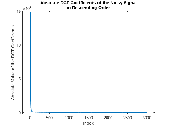
In this section, we show impulse denoising in power line signal using basis pursuit. A signal is said to be compressible with respect to a basis, if the absolute value of its sorted (ascending) coefficients calculated with the basis is exponentially decreasing. In that case, the signal can be well represented with only the largest few coefficients.

As the AC line current signal is sinusoidal, the signal is compressible with respect to the Discrete Cosine Transform (DCT) basis. In contrast, the impulse noise is not compressible in the DCT domain. Due to its impulsive nature, the noise can be better represented using the Identity basis. We can employ basis pursuit with a sensing dictionary built from a combination of DCT and identity bases to separate the underlying signal from the impulsive noise.

Experimental Setup

This example uses main line current signals collected in the BLOND-50 Dataset [5]. This dataset corresponds to the electrical activity in an office space in Germany. In addition to the current and voltage signals that correspond to activities from appliances in the office space, the dataset also includes main line current and voltage signals. During the collection of BLOND-50, connection and disconnection of various appliances and switches resulted in white and impulsive noise in the data. The data was sampled at 50kHz.

This example uses multiple cycles of the raw recorded current signals in the 3-phase power grid from a specific day of the year. The data is in the file lineCurrent.mat, which is included with the example. The 3-phase power grid is characterized by a 120° phase shift between the circuits.

Load the signal from the lineCurrent.mat file. Plot one segment of the recorded noisy line current signal from all 3-phases.

load lineCurrent
Fs = 50e3;
t = (0:(length(I1)-1))/Fs;

figure
tiledlayout(3,1)
nexttile
plot(t,I1)
title("Current Signal From Phase 1")
xlabel("Time (sec)")
ylabel("Current Value (A)")
nexttile
plot(t,I2)
title("Current Signal From Phase 2")
xlabel("Time (sec)")
ylabel("Current Value (A)")
nexttile
plot(t,I3)
title("Current Signal From Phase 3")
ylabel("Current Value (A)")
xlabel("Time (sec)")

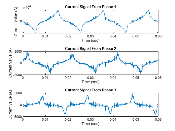
From the plots we can see that the signals from all three phases are affected by impulse noise. The impulsive nature of the noise causes the spiky appearance of the signals.

Generate the basis dictionary A that will be used for basis pursuit.

N = length(I1);

% Generate the sensingDictionary
A = sensingDictionary(Size=N,Type={'dct','eye'});

Calculate the coefficients of the noisy signal from phase 1 in DCT domain.

% Obtain DCT basis matrix
ADCT = subdict(A,1:N,1:N);
% Calculate the DCT coefficients
cDCT = ADCT'*double(I1);

Observe the ordered absolute coefficients of the signal in DCT domain. The plot shows that the DCT coefficients are exponentially decreasing. In other words, the signal can be compressed using a few DCT bases.

figure
sortedcDCT = sort(abs(cDCT),"descend");
plot(sortedcDCT,LineWidth=2)
title({"Absolute DCT Coefficients of the Noisy Signal"; "in Descending Order"})
axis([-200 3200 -2000 max(abs(cDCT))+1000])
xlabel("Index")
ylabel("Absolute Value of the DCT Coefficients")

Figure contains an axes object. The axes object with title Absolute DCT Coefficients of the Noisy Signal in Descending Order, xlabel Index, ylabel Absolute Value of the DCT Coefficients contains an object of type line.

Perform basis pursuit on the noisy current signal using the helper function impulseDenoise and obtain the denoised signal y1.

% Perform impulse denoising
[y1, y2] = helperImpulseDenoise(A,I1,N);

Plot the denoised signal and the separated impulse noise.

% Display the denoised signal and the impulse noise
tiledlayout(3,1)
nexttile
plot(t,I1,LineWidth=2)
xlabel("Time (sec)")
ylabel("Current Value (A)")
title("Noisy Current Signal From Phase 1")
nexttile
plot(t,y1,LineWidth=2)
xlabel("Time (sec)")
ylabel("Current Value (A)")
title("Denoised Current Signal")
nexttile
plot(y2,LineWidth=2)
title("Impulse Noise")
ylabel("Noise Amplitude")
xlabel("Time (sec)")

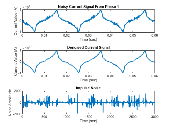
The plots show that basis pursuit successfully separated the current signal from the impulse noise. Repeat the impulse denoising process on the current signals on the remaining two phases.

% Perform impulse denoising on the current signals from phase 2 and 3
[y21, ~] = helperImpulseDenoise(A,I2,N);
[y31, ~] = helperImpulseDenoise(A,I3,N);

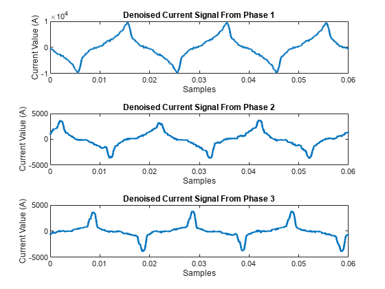
Plot the impulse denoised current signals from all three phases.

figure
tiledlayout(3,1)
nexttile
plot(t,y1,LineWidth=2)
xlabel("Samples")
ylabel("Current Value (A)")
title("Denoised Current Signal From Phase 1")
nexttile
plot(t,y21,LineWidth=2)
xlabel("Samples")
ylabel("Current Value (A)")
title("Denoised Current Signal From Phase 2")
nexttile
plot(t,y31,LineWidth=2)
xlabel("Samples")
ylabel("Current Value (A)")
title("Denoised Current Signal From Phase 3")

Summary

In this example, we demonstrated how sparsity of a signal can be exploited to perform impulse denoising. As the data transmitted in the PLC networks are more vulnerable to impulse noise than Gaussian noise, it is essential to perform impulse denoising to ensure data integrity at the receiver end.

References

[1] Dai, Ronghuo, Cheng Yin, Shasha Yang, and Fanchang Zhang. “Seismic Deconvolution and Inversion with Erratic Data: Seismic Deconvolution and Inversion with Erratic Data.” Geophysical Prospecting 66, no. 9 (November 2018): 1684–1701. https://onlinelibrary.wiley.com/doi/full/10.1111/1365-2478.12689.

[2] Peyré, G. "The numerical tours of signal processing-advanced computational signal and image processing." IEEE Computing in Science and Engineering, 2011, 13(4), pp.94-97. https://hal.archives-ouvertes.fr/hal-00519521/document.

[3] Lampe, L., "Bursty impulse noise detection by compressed sensing," 2011 IEEE International Symposium on Power Line Communications and Its Applications, 2011, pp. 29-34, https://ieeexplore.ieee.org/document/5764411.

[4] Middleton, D. and Institute of Electrical and Electronics Engineers, 1960. An introduction to statistical communication theory (Vol. 960). New York: McGraw-Hill. https://ieeexplore.ieee.org/abstract/document/5312360.

[5] Kriechbaumer, T. & Jacobsen, H.-A. "BLOND, a building-level office environment dataset of typical electrical appliances." Sci. Data 5:180048 https://www.nature.com/articles/sdata201848.

Helper Functions

sparseSignal - This function generates the sparse signal that corresponds to the 1-D ground profile.

function x = sparseSignal(N)
% This function is only intended to support examples in the Wavelet
% Toolbox. It may be changed or removed in a future release.
m = 5; M = 40;
k = floor( (N+M)*2/(M+m) )-1;
spc = linspace(M,m,k)';

% Location of the impulses
idx = round( cumsum(spc) );
idx(idx>N) = [];

x = zeros(N,1);
si = (-1).^(1:length(idx))';
si = si(randperm(length(si)));

% Creating the sparse signal.
x(idx) = si;
x = x .* (1-rand(N,1)*.5);
end

impulseDenoise - This function performs the impulse denoising using basis pursuit.

function [y1, y2] = helperImpulseDenoise(A,y,N)
% This function is only intended to support examples in the Wavelet
% Toolbox. It may be changed or removed in a future release.

% Perform basis pursuit on the measurement y
[XBP,~,~] = basisPursuit(A,y);

% Obtain the denoised current signal using DCT basis
A1mat = subdict(A,1:N,1:N);
y1 = A1mat*XBP(1:N);

% Separate the impulse noise using Identity basis
A2mat = subdict(A,1:N,(N+1):(2*N));
y2 = A2mat*XBP((N+1):end);
end

Signal Deconvolution and Impulse Denoising Using Pursuit Methods

Example 1: Sparse Seismic Deconvolution With Orthogonal Matching Pursuit

Generate Seismic Filter

Sparse Spike Deconvolution With Orthogonal Matching Pursuit

Summary

Example 2: Impulse Denoising in Line Current Using Basis Pursuit

Impulse Denoising Using Basis Pursuit

Experimental Setup

Summary

References

Helper Functions

See Also

Related Topics