GMSK Demodulator

Demodulate GMSK-modulated symbols to set of LLR values or bits

Since R2026a

Libraries:
Wireless HDL Toolbox / Modulation

Description

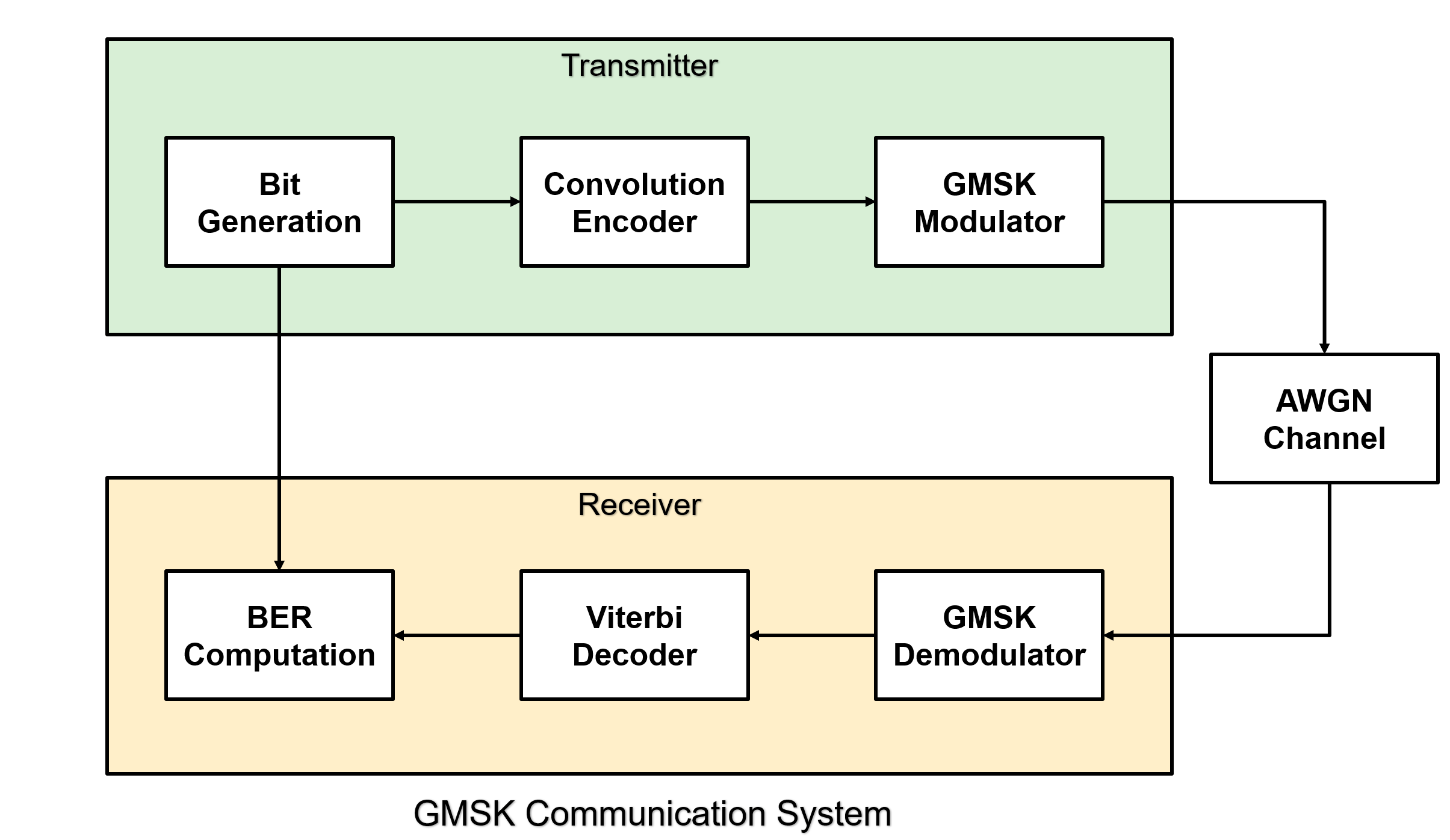
The GMSK Demodulator block demodulates Gaussian minimum shift keying (GMSK) modulated symbols to a set of log-likelihood ratio (LLR) values or data bits. The block accepts complex data symbols and outputs demodulated LLR values or data bits. The block accepts scalar and vector inputs and returns a scalar output. The block interface and architecture are suitable for HDL code generation and hardware deployment.

You can implement GMSK demodulation in systems where efficient bandwidth and power usage are essential, as GMSK modulation is specifically designed to address these requirements. By integrating a GMSK demodulator into such a system, you enable the receiver to take advantage of the modulation’s spectral and power efficiency, ensuring accurate recovery of transmitted data. You can use this block in applications such as global system for mobile communications (GSM), Bluetooth, and satellite communications, where optimizing resources is critical.

Examples

New

Recover Data Bits with GMSK Modulation and Demodulation

Convert data bits into modulated symbols and then recover the original bits through demodulation.

Since R2026a
Open Script

New

Accelerate BER Simulations of GMSK System Using FPGA-in-the-Loop Workflow

Accelerate BER simulations of GMSK system using FPGA-in-loop workflow.

Since R2026a
Open Live Script

Ports

Input

expand all

data — Data symbols
complex scalar | complex column vector

Data symbols, specified as a complex scalar or as a complex column vector. For vector inputs, the vector size must be equal to the number of samples per symbol.

The block supports double and single data types for simulation but not for HDL code generation. For HDL code generation, the input data type must be fixdt(1, WL, FL) with word length WL and fraction length FL not equal to zero. The maximum output word length the block supports is 32 bits.

Data Types: single | double | fixed point
Complex Number Support: Yes

valid — Signal to indicate valid input data
scalar

Signal to indicate valid input data, specified as a Boolean scalar.

This control signal at this port indicates when the sample from the data input port is valid. When the value at this port is 1, the block captures the values on the data input port. When the value at this port is 0, the block ignores the values on the data input port.

Data Types: Boolean

reset — Signal to clear internal states
scalar

Signal to clear internal states, specified as a Boolean scalar. When the value at this port is 1, the block stops the current calculation and clears all internal states.

Dependencies

To enable this port, select the Enable reset input port parameter.

Data Types: Boolean

Output

expand all

data — Output LLR values or data bits
real scalar

Output data bits, returned as a real scalar of LLR values or data bits.

When you set the Decision type parameter to Soft, the output is a scalar of LLR values. For soft-decision type, the output word length depends on the pulse length and the number of samples per symbol.
When you set the Decision type parameter to Hard, the output is a scalar of data bits.

Data Types: single | double | signed fixed point

valid — Signal to indicate valid output data
scalar

Signal to indicate valid output data, returned as a scalar.

This port is a control signal that indicates when the data output port is valid. When the value at this port is 1, the output data samples are available on the data output port.

Data Types: Boolean

Parameters

expand all

To edit block parameters interactively, use the Property Inspector. From the Simulink^® Toolstrip, on the Simulation tab, in the Prepare gallery, select Property Inspector.

Bandwidth time product — Product of bandwidth and symbol time for Gaussian pulse shape
`0.3` (default) | positive scalar value

Product of the signal bandwidth and symbol time for the Gaussian pulse shape, specified as a positive scalar value.

Pulse length (symbol intervals) — Pulse length
`2` (default) | positive integer in the range from 1 to 8

Pulse length, specified as a positive integer in the range from 1 to 8. The pulse length parameter specifies the duration of the Gaussian pulse shape measured in symbol intervals.

Symbol prehistory — Symbol prehistory
`1` (default) | `-1` | vector of –1s or 1s with length equal to L – 1

Symbol prehistory, specified as a scalar or vector of –1s or 1s. The block uses the symbol prehistory before the start of the simulation to estimate the most likely sequence of transmitted data.

For a scalar value, the block expands it to a vector of length L – 1, where L represents the pulse length. You can specify the L value using the Pulse length (symbol intervals) parameter.
For example, if you specify a scalar value -1 and set the Pulse length (symbol intervals) parameter to 4, the block expands this value as [-1 -1 -1].
For a vector value, the block considers the elements in the vector in a reverse chronological order. The vector length must be L – 1.
For example, if you specify a vector input of [-1 1 1] and set the Pulse length (symbol intervals) parameter to 4, the block considers this value as [1 1 -1].

Phase offset (rad) — Phase offset of modulated waveform
`0` (default) | numeric scalar in the range from –2π to 2π.

Phase offset of the modulated waveform in radians, specified as a numeric scalar in the range from –2*π to 2*π.

Samples per symbol — Number of samples per symbol
`4` (default) | positive integer in the range 1 to 8

Number of samples per symbol, specified as a positive integer in the range 1 to 8. The number of samples per symbol represents the upsampling factor from input samples to output samples.

Traceback depth — Traceback depth
`16` (default) | positive integer

Traceback depth, specified as a positive integer. The traceback depth specifies the number of trellis branches that the maximum-a-posteriori (MAP) decoding algorithm uses to construct each traceback path.

For GMSK, the number of correlative states is equal to 2^{L – 1} and there are four phase states, which are 0, π/2, π, 3π/2. Here, L is the pulse length. For a pulse length of 3, you compute the total number of states as 4 × 2^{L – 1}, which equals 16.

Decision type — Decision type
`Soft` (default) | `Hard`

Decision type, specified as Soft or Hard.

When you set the Decision type parameter to Soft, the output is a scalar of LLR values.
When you set the Decision type parameter to Hard, the output is a scalar of data bits.

Enable reset input port — Option to reset signal
`off` (default) | `on`

Select this parameter to enable the reset input port.

Algorithms

expand all

The GMSK Demodulator block uses either hard or soft-decision techniques. Hard demodulation makes a firm choice for each received symbol, while soft demodulation provides likelihood information that enhances error correction, especially in noisy environments. For narrowband, low-throughput systems where GMSK is commonly used, soft demodulation offers significant performance advantages. It typically relies on sequence estimation algorithms such as the soft Viterbi or maximum-a-posteriori (MAP) decoding. Among these, MAP decoding is preferred over the soft output Viterbi algorithm (SOVA) due to its superior error-correcting capability. This block implements the max-log-MAP variant, which achieves an effective balance between computational complexity and decoding accuracy, making it well-suited for hardware-based systems.

To compute soft log-likelihood ratios (LLRs) using the Max-Log-MAP algorithm, calculate and store branch metrics (γ), forward metrics (α), and reverse metrics (β).

Branch Metric Calculation: You compute the branch metrics γ according to the following equation:

$T = \sum_{1}^{s p s} (x_{r} y_{r} + x_{i} y_{i})$
Forward Metric Calculation: Next, you use the γ values to compute the forward metrics α as follows:

$A_{k} = \max [A_{k - 1} + T_{k}]$

You initialize α with:

$A_{0} = {_{- \infty, f o r s \neq 0}^{0, f o r s = 0}$
Reverse Metric Calculation: To calculate the reverse metrics β, you store the γ values and access them as needed:

$B_{k - 1} = \max [B_{k} + T_{k}]$
Log-Likelihood Ratio Calculation: You then calculate the LLR from the stored α and γ values, along with the computed β values:

$L L R = \max_{S_{1}} [A_{k - 1} + T_{k} + B_{k}] - \max_{S_{0}} [A_{k - 1} + T_{k} + B_{k}]$

You can further simplify this calculation as:

$L L R = \max_{S_{1}} [A_{k - 1} + T_{k} + B_{k}] - \max_{S_{0}} [A_{k - 1} + T_{k} + B_{k}]$

Here, S₀ and S₁ represent the sets of state transitions corresponding to bit 0 and bit 1, respectively.

To ensure that these computations work efficiently, you must store both γ and α values according to the specified traceback depth. To optimize hardware efficiency, you implement the K-pointer algorithm, where K is the number of read pointers required in the algorithm. You allocate three memory blocks, each sized according to the traceback depth, to store the input data. You perform the traceback operation to compute the β values required for LLR computation. This approach allows you to read and write in reverse order based on the pointer and the demodulator state, which conserves memory resources.

The following figure illustrates the process of writing, reading, and performing traceback across different input windows during data decoding. While you encounter an initial latency of 4TB cycles, the output data stream is continuous thereafter, ensuring that throughput remains unaffected.

Read, Write, and Traceback Operation

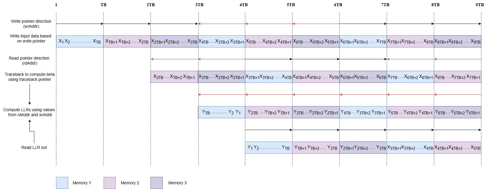
For more information about K-pointer algorithm, see Algorithms.

This approach enables efficient and reliable soft LLR computation in hardware implementations of the Max-Log-MAP algorithm. Hard-decision bit values are defined by rounding the LLR outputs resulting from soft-decision decoding.

Latency

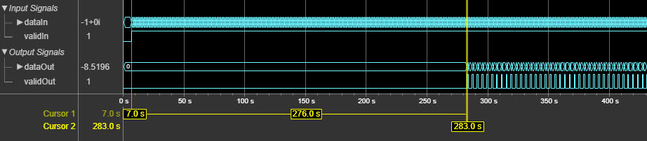
The latency of the block varies with the pulse length, traceback depth, and the input size.

This figure shows a sample output and latency of the GMSK Demodulator block for a scalar input with default configuration. The latency of the block is 276 clock cycles.

GMSK Demodulator Block Latency Default Configuration for Scalar Input

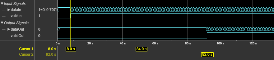
This figure shows a sample output and latency of the GMSK Demodulator block for a vector input with default configuration. The latency of the block is 84 clock cycles.

GMSK Demodulator Block Latency Default Configuration for Vector Input

Performance

The performance of the synthesized HDL code varies with your target and synthesis options. It also varies based on the pulse length, traceback depth, and the input size.

This table shows the resource and performance data synthesis results of the block for a 4-by-1 vector input and a scalar input, respectively, in the default configuration. The generated HDL code targets to the AMD^® Zynq^® UltraScale+™ MPSoC - ZCU102 Evaluation Board.

Input Type	CLB LUTs	CLB Registers	DSPs	Block RAMs	Maximum Frequency in MHz
Scalar	6228	3631	12	0	272.33
Vector (4-by-1)	6947	4461	39	0	272.33

References

[1] Anderson, John B., Tor Aulin, and Carl-Erik Sundberg. Digital Phase Modulation. New York: Plenum Press, 1986.

Extended Capabilities

expand all

C/C++ Code Generation
Generate C and C++ code using Simulink® Coder™.

This block supports C/C++ code generation for Simulink accelerator and rapid accelerator modes and for DPI component generation.

HDL Code Generation
Generate VHDL, Verilog and SystemVerilog code for FPGA and ASIC designs using HDL Coder™.

HDL Coder™ provides additional configuration options that affect HDL implementation and synthesized logic.

HDL Architecture

This block has one default HDL architecture.

HDL Block Properties

ConstrainedOutputPipeline	Number of registers to place at the outputs by moving existing delays within your design. Distributed pipelining does not redistribute these registers. The default is `0`. For more details, see ConstrainedOutputPipeline (HDL Coder).
InputPipeline	Number of input pipeline stages to insert in the generated code. Distributed pipelining and constrained output pipelining can move these registers. The default is `0`. For more details, see InputPipeline (HDL Coder).
OutputPipeline	Number of output pipeline stages to insert in the generated code. Distributed pipelining and constrained output pipelining can move these registers. The default is `0`. For more details, see OutputPipeline (HDL Coder).
SynthesisAttributes	Specifies the synthesis attributes for the blocks and block output signals in the model. The generated HDL code contains these attributes. For more information, see SynthesisAttributes (HDL Coder).

Restrictions

You cannot generate HDL for this block inside a Resettable Synchronous Subsystem (HDL Coder).

Version History

Introduced in R2026a

GMSK Demodulator

Description

Examples

Recover Data Bits with GMSK Modulation and Demodulation

Accelerate BER Simulations of GMSK System Using FPGA-in-the-Loop Workflow