HDL Implementation of Digital Predistorter with LMS Coefficient Estimation
This example shows how to implement a digital predistorter (DPD) with least mean squares (LMS) based coefficient estimation, which is optimized for HDL code generation and hardware implementation. This example expands on the HDL Implementation of Digital Predistorter example for computing DPD coefficients on an FPGA instead of a processor.
This example contains two Simulink® models.
HDLDPDwithLMSCoeffExample— Use this model to perform predistortion using an adaptive LMS coefficient estimator that estimates coefficients dynamically. This model replaces the C/C++ code generatableRPEM Coeff Estimationsubsystem of the HDL Implementation of Digital Predistorter example with an HDL-compatibleLMS Coefficient Estimatorsubsystem.HDLDPDwithPreCalculatedCoeffExample— Use this model to perform predistortion using pre-calculated coefficients.
These example models support Normal and Accelerator simulation modes. For more information about DPD, see Adaptive DPD Design.
Run this command to open the high-level architecture of the HDL DPD with LMS coefficient estimation.
modelname = 'HDLDPDwithLMSCoeffExample';
open_system(modelname);
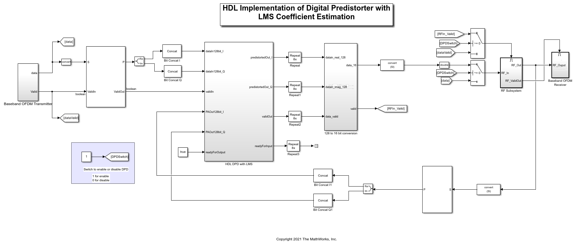
Model Architecture
The Baseband OFDM Transmitter subsystem generates a 16 bit complex baseband orthogonal frequency division multiplexed (OFDM) signal at a sample rate of 15.36 MHz.
The DPD_LMS subsystem of the HDL DPD with LMS subsystem accepts the 16 bit complex data that is generated from the Baseband OFDM Transmitter subsystem and the 16 bit complex data that is generated from the RF Subsystem subsystem. The HDL DPD with LMS subsystem performs DPD using the LMS-based coefficient estimation and returns a 16 bit complex predistorted data at a sample rate of 15.36 MHz.
When you enable the DPDSwitch in the model, the RF Subsystem subsystem accepts 16 bit complex predistorted data from the HDL DPD with LMS subsystem. Otherwise, the subsystem accepts data from the Baseband OFDM Transmitter subsystem as input I and Q samples. The power amplifier (PA) accepts these I/Q samples that are upsampled to 2.4 GHz. The PA is preloaded with the coefficient matrix based on the standard-compliant LTE signal with a sample rate of 15.36 MHz. These PA coefficients are stored in a MAT-file, and these values are loaded while initializing the example.
In the other path, the data is passed through a low noise amplifier (LNA) and is down-converted before providing to the DPD_LMS subsystem in the HDL DPD with LMS subsystem. The Baseband OFDM Receiver subsystem collects the down-converted data and provides it as an input to the OFDMRx function.
For more information about the Baseband OFDM Transmitter, RF Subsystem, and Baseband OFDM Receiver subsystems, see the HDL Implementation of Digital Predistorter example.
Open the HDL DPD with LMS subsystem.
load_system(modelname);
open_system([modelname '/HDL DPD with LMS']);
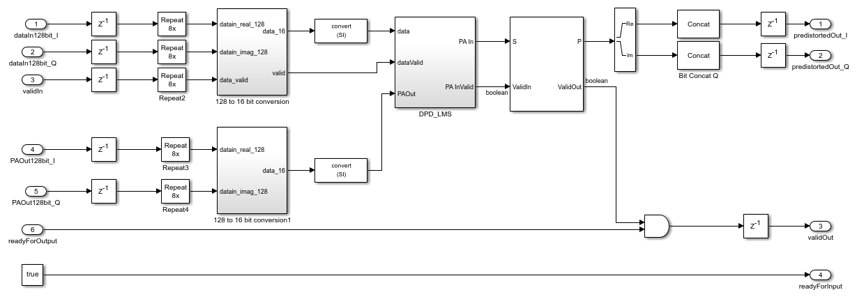
HDL DPD with LMS Coefficients Estimation
The HDL DPD with LMS subsystem performs digital predistortion on 16 bit complex input data that is generated from the Baseband OFDM Transmitter and RF Subsystem subsystems. The DPD_LMS subsystem uses the Digital Predistorter and Least Mean Square Coefficient Estimator subsystems to perform digital predistortion with LMS coefficients.
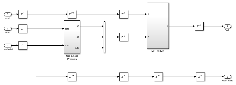
Digital Predistorter
The Digital Predistorter subsystem distorts the 16 bit complex input data using the coefficients that are estimated by the LMS Coefficient Estimator subsystem. The DPD design in this example is similar to the HDL Implementation of Digital Predistorter example, which is optimized for memory depth 3 and polynomial degree 3. The input data is placed in a shift register and multiplexed to form a vector based on the memory depth. Then, the vector is concatenated with the nonlinear products of the data depending on the polynomial degree. This concatenation forms a vector of 9 elements, which equals the memory depth times the degree. The dot product of the obtained vector and estimated coefficients provides the predistorted input that is fed as input to the RF Subsystem subsystem when you enable the DPDSwitch. Open the Digital Predistorter subsystem.
load_system(modelname);
open_system([modelname '/HDL DPD with LMS/DPD_LMS/Digital Predistorter']);
LMS Coefficient Estimator
When PA characteristics vary over time and different operating conditions, using an adaptive estimation algorithm that runs on an FPGA to estimate the inverse of the PA is necessary. In this example, a hardware-friendly estimation algorithm based on the LMS method is considered due to its simple architecture and easier implementation on hardware with less resources compared to other estimation algorithms such as recursive least squares (RLS) and recursive prediction error method (RPEM). The LMS Coefficient Estimator subsystem estimates the DPD coefficients from the outputs of the Digital Predistorter subsystem (the PA input) and the PA output of the RF Subsystem subsystem. Similar to the Digital Predistorter subsystem, the LMS Coefficient Estimator subsystem also operates at 15.36 MHz. For memory depth 3 and polynomial degree 3, the LMS Coefficient Estimator subsystem estimates a total of 9 coefficients. Open the LMS Coefficient Estimator subsystem.
load_system(modelname);
open_system([modelname '/HDL DPD with LMS/DPD_LMS/LMS Coefficient Estimator']);
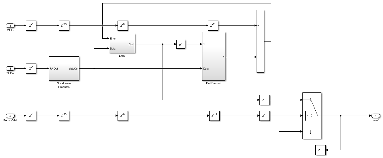
The PA output data from the RF Subsystem subsystem is placed in a shift register based on the memory depth, which is 3. Then, this vector is concatenated with the nonlinear products of the PA output data depending on the polynomial degree, which is 3. This concatenation forms a vector of 9 elements, which equals the memory depth times the degree. The LMS subsystem estimates the coefficients such that the error is minimal between the PA input data and the PA output data. The Dot product subsystem performs the dot product of the conjugate of the estimated coefficients and the concatenated PA output data. To send out the estimated coefficients based on PA In Valid, the example uses a switch. When the PA In Valid is high (1), this subsystem sends the current estimated coefficients. Otherwise, the subsystem sends the previously estimated coefficients.
Verification and Results
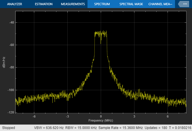
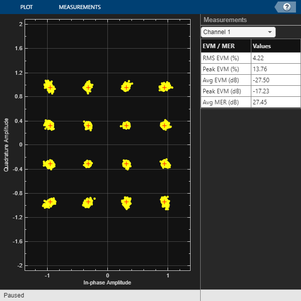
Run the HDLDPDwithLMSCoeffExample model. By default, the DPDSwitch is enabled. If you disable it, the error vector magnitude (EVM) and spectral regrowth in adjacent channels increase. The constellation and spectrum analyzer diagrams show the results of running the HDLDPDwithLMSCoeffExample model with the DPD enabled.
sim(modelname);
 Estimating carrier frequency offset ...

 First four frames are used for carrier frequency offset estimation.

 Estimated carrier frequency offset is 1.129420e+00 Hz.

 Detected and processing frame 5
------------------------------------------

 Header CRC passed

 Modulation: 16QAM, codeRate=1/2 and FFT Length=128

 Data CRC passed

 Data decoding completed
------------------------------------------

 Detected and processing frame 6
------------------------------------------

 Header CRC passed

 Modulation: 16QAM, codeRate=1/2 and FFT Length=128

 Data CRC passed

 Data decoding completed
------------------------------------------
HDL Code Generation and Implementation Results
To check and generate HDL code for this model, you must have the HDL Coder™ product. To generate HDL code and a testbench for the HDL DPD with LMS subsystem, use the makehdl and makehdltb commands.
The HDL DPD with LMS subsystem is synthesized on the Xilinx® Zynq® Ultrascale RFSoC ZCU111 evaluation board. The frequency obtained after place and route is about 520 MHz. This table displays the post place and route resource utilization results for a 16 bit complex input.
F = table(...
    categorical({'Slice LUT'; 'Slice Registers';'DSP'}), ...
    categorical({'3815'; '8185'; '120'}), ...
    categorical({'425280'; '850560'; '4272'}), ...
    categorical({'0.90'; '0.96'; '2.81'}), ...
    'VariableNames', ...
    {'Resources','Utilized','Available','Utilization (%)'});
disp(F);
       Resources       Utilized    Available    Utilization (%)
    _______________    ________    _________    _______________

    Slice LUT            3815       425280           0.90
    Slice Registers      8185       850560           0.96
    DSP                  120        4272             2.81
DPD with Pre-calculated Coefficients
To perform digital predistortion with pre-calculated coefficients, use the HDLDPDwithPreCalculatedCoeffExample model and the preCalculatedCoeff MAT file containing pre-calculated coefficients. These coefficients are generated using the HDLDPDwithLMSCoeffExample model.
To create a new set of coefficients for any other PA settings, modify the parameters of the PA in the HDLDPDwithLMSCoeffExample model according to your requirement and run the model. If you already have a set of estimated coefficients to perform digital predistortion, replace the coefficients in preCalculatedCoeff MAT file and run the HDLDPDwithPreCalculatedCoeffExample model.
modelname = 'HDLDPDwithPreCalculatedCoeffExample';
open_system(modelname);

Verification and Results
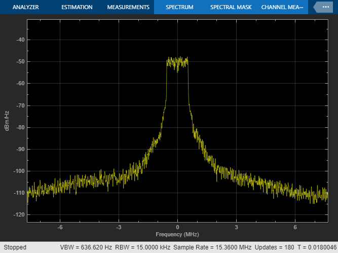
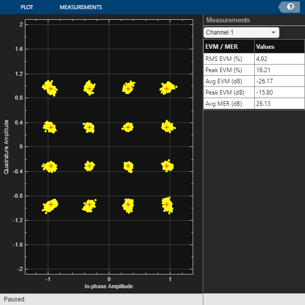
Run the HDLDPDwithPreCalculatedCoeffExample model. By default, the DPDSwitch is enabled. If you disable it, the EVM and spectral regrowth in adjacent channels increase. The constellation and spectrum analyzer diagrams show the results of running the HDLDPDwithPreCalculatedCoeffExample model with the DPD enabled. You can see that when using DPD with pre-calculated LMS coefficients, the spectrum and constellation remain intact.
sim(modelname);
 Estimating carrier frequency offset ...

 First four frames are used for carrier frequency offset estimation.

 Estimated carrier frequency offset is -2.901742e-01 Hz.

 Detected and processing frame 5
------------------------------------------

 Header CRC passed

 Modulation: 16QAM, codeRate=1/2 and FFT Length=128

 Data CRC passed

 Data decoding completed
------------------------------------------

 Detected and processing frame 6
------------------------------------------

 Header CRC passed

 Modulation: 16QAM, codeRate=1/2 and FFT Length=128

 Data CRC passed

 Data decoding completed
------------------------------------------
HDL Code Generation and Implementation Results
To check and generate HDL code for this model, you must have the HDL Coder™ product. To generate HDL code and a testbench for the HDL DPD subsystem, use the makehdl and makehdltb commands.
The Digital Predistorter with pre-calculated LMS coefficients subsystem is synthesized on a Xilinx® Zynq® Ultrascale RFSoC ZCU111 evaluation board. The frequency obtained after place and route is about 550 MHz. This table displays the post place and route resource utilization results for a 16 bit complex input.
F = table(...
    categorical({'Slice LUT'; 'Slice Registers';'DSP'}), ...
    categorical({'1522'; '2416'; '42'}), ...
    categorical({'425280'; '850560'; '4272'}), ...
    categorical({'0.36'; '0.28'; '0.98'}), ...
    'VariableNames', ...
    {'Resources','Utilized','Available','Utilization (%)'});
disp(F);
       Resources       Utilized    Available    Utilization (%)
    _______________    ________    _________    _______________

    Slice LUT            1522       425280           0.36
    Slice Registers      2416       850560           0.28
    DSP                  42         4272             0.98