搜索
 A small MATLAB GPT that groks integer addition
Duncan Carlsmith, Department of Physics, University of Wisconsin-Madison
Introduction
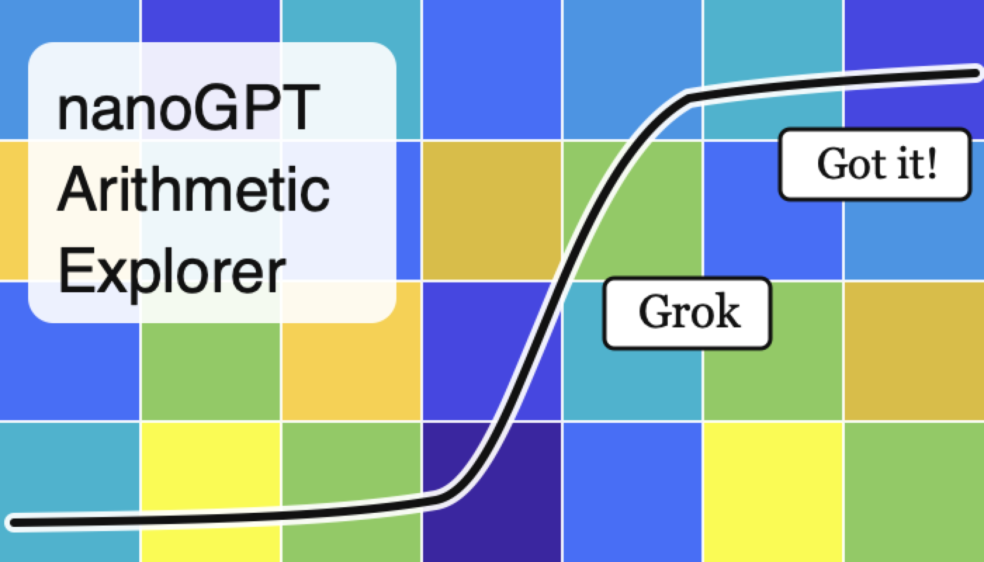
My prior post A miniature GPT language model as a MATLAB Live Script provides a small character-level GPT in MATLAB and trains it on Shakespeare. Language modeling is intractable in the sense that there is no exact answer to grade against; the model is judged by whether its output reads plausibly. This companion Live Script applies the same architecture to a problem with a clear success metric. The goal of training is for the model to discover/get/“grok” an exact algorithm for integer addition in any base (e.g., binary, decimal, and hexadecimal). With this script, you can watch a “grok,” the model suddenly “getting” addition, happen in real time and in detail- very fun if you are like me, hardly an expert!
Addition is easy except for the carry. The digit in a column is the column sum modulo the base. The carry couples columns: a carry out of one column feeds the next, and consecutive carries chain groups of columns together. The script grades the model on held-out problems sorted by the length of the longest carry chain, so the per-chain accuracy curves show exactly where and how the model succeeds. One observes the model first grok single carries, then singles and doubles, and so on, up to the maximum for the range of digits presented during training. In representing a finite range of numbers, the distribution of carry chain lengths depends on the base, as does the number of essential tokens. Hence, although the essence of addition is base-independent, the learning curves are different for different bases.
As is well known, the grok duration can be very short or gradual, depending on exactly how the addition problem is posed when presented to the model and if a random or structured learning curriculum is used. The script demonstrates that since a random number generator based on a seed is used to generate training samples, the time and even existence of a grok in a prescribed length set of training steps fluctuates, sometimes wildly, but for the same seed, and training is reproducible deterministically to machine precision. Comparative studies of the efficacy of different model sizes, problem presentation formats, and training curricula require statistical analysis and are not attempted by this script.
The Live Script is organized as five experiments. The first trains naively on random problems and can show a vexing carry stall - a partial grok. The next two use a difficulty curriculum that orders training from short carry chains to long ones, and a scratchpad format that writes each column's digit and carry explicitly so the carry is a token in context rather than something inferred. The fourth combines both. The fifth trains one model on a mix of bases, each problem labeled with its base, and tests a base never seen in training; the base-independent column sum transfers to the new base, but the base-specific carry threshold does not. Each experiment displays a precomputed figure by default. Each also has a "Try this" switch that retrains it live with your own base, digit count, model size, and seed. A set of challenges asks the reader to extend the work, for example, to test length generalization or study subtraction together with addition.
The engine that does the training and evaluation is a set of MATLAB functions shipped with the script and usable on their own from the Command Window, independent of the Live Script. An accompanying guide documents them for readers who want to understand the details or run their own experiments. The script and engine were built with Claude (Anthropic) working with MATLAB R2026a on my own MacBook with an M1 chip through an ngrok command server, the agentic context described in my prior posts. No GPU or API is used.
References
Duncan Carlsmith (2026). nanoGPT Arithmetic Explorer (https://www.mathworks.com/matlabcentral/fileexchange/184054-nanogpt-arithmetic-explorer), MATLAB Central File Exchange. Retrieved June 11, 2026.
Conflict of interest
The author declares he has no financial interest in MathWorks or Anthropic. This article is informational and does not constitute an endorsement by the University of Wisconsin-Madison of any vendor or product. Claude is a trademark of Anthropic. MATLAB is a trademark of MathWorks.
I've been confused trying to write (or have an AI write) the .m (Live) text format from scratch for various reasons using .mlx format exported with the IDE as .m (old) and .m (LIve). Of course, one problem is the .m and .m (Live) files have the same name,causing confusion and requiring renaming, but repeatedly, after sussing out and following all conventions for headings and latex etc in .m (LIve), my .m (Live) files would not open as .mlx in the IDE. I think I've found the answer by trial and error and comparison and don't know it is documented. Add at the end
%[appendix]{"version":"1.0"} %--- %[metadata:view] % data: {"layout":"inline"} %---
This seems to trigger the IDE to recognize this is a .m (Live). Woohoo! This is a LOT easier than writing .mlx zip packages from scratch.
Have there been some changes made to the ThinkSpeak graphs? I am unable to change the number of days displayed, nor the number of data points to display. I did have them display 5 days, but now they are showing 14 days even though the setting is 5. I tried logging out and back in, but to no avail. Thanks.
var = yes;
86%
var=no;
6%
I don't mind either way
8%
765 个投票
<80 characters
14%
80 characters
25%
100 characters
22%
120 characters
16%
>120 characters
15%
something else (comment below)
9%
198 个投票
camelCase (variableName)
39%
PascalCase (VariableName)
12%
no capitalization (variablename)
4%
snake_case (variable_name)
27%
It varies for me
18%
802 个投票
Many widely cited code style guides originate from large-scale software engineering contexts: multi-developer teams, large codebases, separate reviewers, and tooling-driven workflows. While those constraints are valid in their domain, they often map poorly onto scientific and engineering scripting as it is typically practiced with MATLAB.
In laboratory and engineering environments, code serves a different role. It is frequently written by individuals or small groups, and then iteratively modified, copied, adapted, and extended as part of an evolving problem-solving process. In this context, the primary priorities are not strict stylistic consistency or tooling compatibility, but rather:
- maintaining clarity of underlying structure,
- minimizing the risk of errors during modification, and
- supporting rapid comprehension of mathematically or logically dense code.
This raises the question: should fixed line-length limits be replaced by context-aware principles? Could these be supported by a suitable AI tool?
The following proposal outlines a small set of heuristics governing line length, based on observations of real-world MATLAB usage, particularly for numerically intensive and structurally rich code. These heuristics aim to:
- preserve and expose meaningful structure (e.g. systems of equations, tables, repeated patterns)
- avoid formatting that obscures relationships or introduces errors, and
- treat different kinds of code (logic vs. data vs. structured expressions) appropriately.
Scope
These principles apply to scientific and engineering scripting, particularly:
- MATLAB-like environments
- numerically or structurally dense code
- monolithic or semi-monolithic workflows
- code that is frequently modified, copied, and adapted
They are not intended for large-scale commercial software engineering, where different constraints dominate.
Core Objective
Line length and formatting should maximize comprehension, structural clarity, and correctness under modification, rather than enforce arbitrary limits.
Hierarchy of Heuristics
Higher-numbered heuristics take precedence over lower-numbered ones.
1) Reasonable Line Length
Code intended for reading should use a reasonable line length, guided by:
- human visual comprehension when scanning
- clarity of expression
- preservation of logical units
This would tend toward 70-100 characters per line, depending on the density.
2) Preserve Semantic Integrity of Lines
Line breaks must not split code in ways that degrade understanding.
Avoid:
- dangling fragments
- very short continuation lines
- separation of tightly coupled elements
- etc.
Prefer:
- keeping logically cohesive expressions intact
- breaking only at clear structural boundaries
One slightly longer line is preferable to two poorly structured lines.
3) Treat Data as Data (Not Prose/Code)
Code that primarily represents data rather than logic is not intended for sequential reading.
This includes:
- large numeric vectors
- lookup tables
- pasted datasets
- etc.
Such code:
- may exceed line length limits without restriction
- should prioritize density and structural stability
- is assumed to be accessed via search or indexing rather than visual parsing
Readability is not the objective; retrievability and integrity are. Yes, this intentionally rejects the enterprise concept that data must be separate from code, instead replacing it with the concept that the IDE should support what some real-world users actually use, for example by formatting/aligning/showing data differently.
4) Preserve and Expose 2D Structure
If code encodes a logical, mathematical, or tabular structure with inherent spatial relationships, it should be represented accordingly.
This includes:
- systems of equations
- tabulated data
- repeated structured expressions
- etc.
Requirements:
- alignment should be used where it improves comprehension
- patterns should be visually apparent
- deviations from patterns should be easily detectable
This principle should be applied strongly, tending toward mandatory use where feasible.
Exception
If a structure would become impractically wide, a compromise representation may be used.
Breaking meaningful spatial structure is considered harmful to comprehension and correctness.
5) Preserve Structural Consistency Across Similar Code
Code segments representing similar or related logic should be expressed in consistent structure and layout.
This applies to:
- repeated formulas
- analogous computations
- structurally similar transformations
- etc.
Consistency enables:
- rapid comparison
- detection of inconsistencies
- safer modification
Similar logic should be represented in similar ways.
Meta-Principles
A. Structure Over Style
Line lengths should reflect the underlying structure of the problem, not conform to arbitrary limits.
B. Correctness Over Convention
Avoid line lengths and formatting that:
- obscures patterns
- hides inconsistencies
- increases the risk of modification errors
C. Optimize for Modification
Code in this domain is frequently:
- edited
- duplicated
- adapted for n
- extended
- commented-out for testing different versions
- etc
Line lengths should reduce the likelihood of errors during these operations, for example by keeping atomic concepts on the same line rather than splitting them up.
D. Anomaly Visibility
Formatting should make unexpected deviations immediately visible.
E. Tool Support
An intelligent tool should:
- respect and preserve structural layout
- avoid rigid line-length enforcement
- detect patterns and inconsistencies
- assist rather than constrain the programmer
I would be interested to hear how well these ideas match others’ experience, particularly in scientific or engineering workflows.
See also:
Cross posted from YouTube: Build, test, and deploy an embedded system with the help of AI, without sacrificing engineering rigor.
In this MATLAB Tech Talk, learn how to use an agentic AI tool alongside MATLAB® and Simulink® to design and control an inverted pendulum (Quanser Qube-Servo and Raspberry Pi®).
Instead of “vibe coding,” focus on a structured, model-based workflow that includes defining requirements, reusing verified models and toolboxes, designing controllers (MPCs), and validating through simulation and staged testing. The key idea is simple: AI is most powerful when it works within proven engineering processes, helping you move faster while keeping results transparent, traceable, and trustworthy.
Learn more about Agentic AI for MATLAB and Simulink: https://bit.ly/4tKcUTy
It used to be possible to flag solutions, e.g. as "hack/cheat", "needs rescoring", and so on. Ever since the update to Cody's design, this has been missing. Are there any plans to bring it back?
I would like hints in Cody.
33%
I would not like hints in Cody.
67%
3 个投票
Is there anywhere to get help for the Cody problems? I am having trouble solving some of them, and I wish we could get hints. If not, is that a feature that could be added?
The problem with Trigonomety is: they do not tell you why you need to know what Cos, Sin, or Tan is, or what they are used for. It seems like a mystery, because you do not know why you need to know it, or what they are used for at all.
A miniature GPT language model MATLAB Live Script
Duncan Carlsmith, Department of Physics, University of Wisconsin-Madison
I have built many MATLAB Live Scripts that take some piece of physics, computation, or machine learning apart so a student can see how it works. The newest one builds, trains, and runs a small GPT language model and was built with AI assistance and may interest readers of this forum.
The model is a MATLAB implementation modeled on nanoGPT, a compact GPT (Generative Pre-trained Transformer) written in Python by Andrej Karpathy and released under the MIT license. This small model is a GPT in each respect: it is generative, producing text one character at a time rather than classifying text; it is pre-trained, trained once on a body of text so that the trained weights can then be reused; and it is a transformer, built from the stack of masked self-attention and feed-forward layers described in more detail in the Live Script Background section. The script trains a character-level model with about 112,000 parameters, two transformer blocks, and one or four attention heads. It is trained on an approximately one-million-character corpus of Shakespeare in roughly twenty minutes on a laptop and, remarkably, generates Shakespeare-flavored text one character at a time. The model parameter count and training corpus pale in comparison to frontier models with estimated parameter counts of order one trillion trained and tens of trillions of tokens. The aim of the Live Script is explanation, not performance.
MATLAB implementation
The training script is vectorized: weights are created as dlarray objects, the loss is computed under dlfeval, and a single call to dlgradient returns the gradient with respect to every weight. The attention of a whole batch of sequences is computed in one pagemtimes call rather than a loop. The autodiff and the batched array arithmetic are what make training on a laptop practical.
A note on the development
The script, the model class, and the trainer were built with Claude (Anthropic), starting with the Python and working with MATLAB R2026a on my own machine through an ngrok command server.
Try this and challenge options
The script ships with the Shakespeare text and one pre-trained model. It also includes an optional section that downloads three public-domain novels from Project Gutenberg — Conan Doyle, Wells, Austen — strips the license boilerplate, and aggregates them into a single corpus, so a student can train a model that writes in a different voice. A model trained on novels does not sound like one trained on Shakespeare, and that difference is the most direct lesson the script offers about what these models actually learn. Several challenges are offered to expand the model and the demonstration.
The submission is on the MATLAB Central File Exchange: Duncan Carlsmith (2026). nanoGPT Explorer (https://www.mathworks.com/matlabcentral/fileexchange/183953-nanogpt-explorer), MATLAB Central File Exchange. Retrieved May 24, 2026.
Conflict of interest
The author declares he has no financial interest in MathWorks or Anthropic. This article is informational and does not constitute an endorsement by the University of Wisconsin-Madison of any vendor or product. Claude is a trademark of Anthropic. MATLAB is a trademark of MathWorks.
talks about how GeForce has become deprioritized by Nvidia, and
The chatter from the grapevine is that we won't see any new GPUs from Nvidia this
year at all — not one — and that's very rare (in fact it hasn't happened in three
decades). This is because Nvidia needs all the chips it can get — and perhaps more
to the point, all the video RAM — for AI graphics cards which are far more
profitable than consumer models.
Soon, Mathworks will be facing a choice: continue to support only expensive Nvidia AI offerings -- or diversify to support alternative GPUs as well.
By the way: Nvidia AI units cost $US7.8 million dollars. https://www.tomshardware.com/tech-industry/artificial-intelligence/nvidias-memory-costs-soar-485-percent-latest-ai-systems-now-cost-usd7-8-million-to-build-memory-now-comprises-25-percent-of-the-total-cost-rubin-gpus-a-mere-usd50-000-apiece
Which alternative GPUs would you most like to see supported?
- Unfortunately, I hear that Apple provides poor support for information on really using their "silicon" GPUs in any way other than Apple's pre-packaged computation libraries. The Apple attitude is apparently that anything that is not already nailed down by documentation is fair game for changing in the future, and that documenting how the GPUs really work would constitute nailing them down, supposedly "destroying" Apple's creativity. Exception: Apple is known to work with major gaming studios (but only the major ones.)
- The Apple silicon series of GPU does not provide any 64 bit operations, so 64 bit support would require emulating 64 bits in software. Nvidia is famous for internally implementing 64 bit support in terms of 32 bit operations, at 1:32 of the speed -- but on the other hand select Nvidia devices operate 64 bit operations at 1:24 or even 1:8 (a small number of devices) through hardware acceleration units. People who need 64 bit operations have the option of shopping very carefully in Nvidia's line to get faster 64 bit processing.
- OpenCL sounds cool and "open". Unfortunately it turns out that a lot of OpenCL operations are optional, so efficient OpenCL libraries would need to be tuned to the exact hardware series.
- OpenCL is not supported on semi-recent MacOS Intel or Apple Silicon series
- I seem to recall hearing that OpenCL is no longer supported by Nvidia either
Background: I've been using Claude Code with the MATLAB MCP Core Server and Simulink Agentic Toolkit for powertrain simulation work — building PMSM FOC controllers, Simscape thermal models, and suspension systems. After a few sessions I noticed a large fraction of my context window was being consumed by output that's useful to a human but not to an LLM: aligned whos tables, repeated solver warnings (one per timestep), deep call stacks with HTML hyperlinks, Simulink build logs, etc.
What I built: A transparent Python stdio proxy that sits between Claude Code and matlab-mcp-core-server. It intercepts tool responses and applies 14 MATLAB/Simulink/Simscape-specific compression rules before the output reaches Claude's context window. Requests are never touched — only responses.
Example reductions:
- whos variable table → 74% reduction (1,800 chars → 189 chars)
- Repeated solver warnings (×10 RCOND warnings) → 71% reduction
- Large array auto-display (1000-row vector) → 85% reduction
- Simulink build log → 56% reduction
- DOE progress loop (55 points) → 79% reduction
- Session average: 48–66% reduction
It also fixes the simulink session attach problem. Without --initialize-matlab-on-startup=true on the matlab server, the simulink server's 30-second discovery window expires before MATLAB is ready. The proxy config includes this flag and documents why it's necessary (root cause traced through server logs).
Validated on: A 2-DOF Simscape quarter-car active suspension model built entirely via model_edit from the SATK — active PD controller achieved 61.7% lower peak chassis velocity and settled 34% faster than passive.
Includes 37 unit tests, full HTML documentation, and the validated Simscape model. Would be interested to hear if others have run into the same output verbosity issues and what workarounds you've tried.
Prototyping MATLAB code in Claude's container with Octave
Duncan Carlsmith, Department of Physics, University of Wisconsin-Madison

Fig. 1: Simulated rigid molecules trajectories
When working with AI to develop MATLAB code for a chaotic-dynamics simulator, I discovered a useful workflow trick: Claude's container ships with GNU Octave. Claude can write .m files and execute them directly, as it can Python, getting fast feedback before you ever push to your local system. The related workflow described here may be possible using any agentic AI offering access to Octave.
The code simulates a classical 2D monatomic or diatomic (rigid or flexible) molecule undergoing a volume compression and compares the adiabatic coefficient in the simulation to the predictions of the ideal gas model and classical thermodynamics, assuming equipartition of energy between the translational, rotational, and vibrational degrees of freedom. Energy is injected by the moving container wall to various degrees of freedom during collisions, and the goal is to see how well the degrees of freedom thermalize through wall collisions alone without intermolecular collisions, and to study wall shape effects. The simulation uses an impact dynamics model for the collisions and tightly controlled state propagation.
My setup includes Claude, an ngrok link to speed up file transfer between a chat container and my local file system, and MATLAB MCP, enabling Claude to push and run MATLAB R2025b and collect output. I decided to first develop in Python entirely in the container, telling Claude to think in advance about porting to MATLAB. This approach allowed Claude to debug quite a package of Python code without the overhead of transferring code and results to and from my system. At various stages, we backed up the Python along with status reports to my filesystem in case the chat failed.
The next stage was to port to MATLAB. When Claude just launched into testing the MATLAB code with Octave in its container, I was taken aback - I hadn’t ever thought of that or known it was a built-in option. We proceeded to make floating-point comparisons of the Python and Octave simulation outputs (which agreed to ~1e-13) to debug the Octave. Finally, we simply transferred about 30 files of Octave/MATLAB code to my filesystem and verified it worked.
The version problem
Claude's container runs Octave 8.4.0, released in late 2023. The current Octave is 11.1.0, released February 2026. Octave is actively maintained, with three or four releases per year. Newer classdef improvements, advances with sparse/diagonal matrices, and various function flags available in 11.1 are lacking in 8.4. For my simulation code, none of this turned out to matter.
Why not just upgrade?
According to Claude, “the container is Ubuntu 24.04 LTS, and its repositories only offer 8.4.0. A standard apt-get install chain failed in interesting ways — Ubuntu's security archive sometimes drops point-version .deb files that the local package index still references, breaking unrelated dependency chains. The openssh-client package got 404'd, which cascaded through openmpi-bin, stopping the install.” Claude suggested “building from source (45+ minutes of compile, plus C++20 and Fortran toolchains), a third-party PPA, or Flatpak (which isn't installed).” My answer was: “I don’t understand all that gobbledygook. Live with 8.4, but write code that will also work in modern MATLAB.”
Octave 8.4 handles array operations, slicing, broadcasting, structs, .mat file I/O via load/save, anonymous functions, fzero and other root-finders, ODE solvers, +package/ namespace folders, sparse matrices, and basic plotting. For our project — a wall-collision simulator with a Forest-Ruth symplectic integrator and Brent's method root-finding — every line of Python code ran identically in MATLAB. The numerical answers differed at the floating-point-precision level (Octave's fzero and MATLAB's fzero round slightly differently, apparently).
Gotchas
A few pitfalls were encountered that you might note if you try this workflow.
1. Nested function definitions inside loops or after executable code
Octave is relaxed about where you put helper function blocks. MATLAB R2025b is strict: local functions go at the end of a file, not inside another function body or — fatally — inside a for loop. I had written:
for i = 1:n
if condition
function f = f_trial(t) % LEGAL in Octave, ERROR in MATLAB
...
end
root = fzero(@f_trial, ...);
end
end
MATLAB rejected this with "Function definition is misplaced or improperly nested." The fix is to move helpers to the end of the file as proper local functions, and use anonymous functions for closures over loop-local variables:
for i = 1:n
if condition
r0 = snapshot_r; % capture in loop scope
f_trial = @(t) helper(t, r0, ...); % captures at creation
root = fzero(f_trial, ...);
end
end
function f = helper(t, r0, ...) % at file end
...
end
2. MATLAB's arguments...end validation block
A MATLAB feature for argument typing and defaults is unsupported in Octave. The modern MATLAB style:
function log = simulate(state, schedule, opts)
arguments
state struct
schedule struct
opts.N_max (1,1) double = 200000
opts.verbose (1,1) logical = false
end
% opts.N_max and opts.verbose available, types and sizes validated
...
end
Octave's parser doesn't recognize the arguments keyword. The fallback is old-style manual parsing:
function log = simulate(state, schedule, varargin)
N_max = 200000;
verbose = false;
for k = 1:2:numel(varargin)
switch varargin{k}
case 'N_max', N_max = varargin{k+1};
case 'verbose', verbose = varargin{k+1};
end
end
...
end
3. Hardcoded paths
Not an Octave-specific problem, but Claude's container has different paths than your local filesystem. Resolve data files relative to the script:
this_dir = fileparts(mfilename('fullpath'));
data = load(fullfile(this_dir, 'comparison', 'data.mat'));
4. Variable name collision
Again, not an Octave-specific problem, but variable name collisions (with Python objects in your workspace, or stale function caches after Claude pushes a new file) can cause confusing errors. clear all resets both.
5. Floating-point differences that get amplified
Octave's fzero and MATLAB's fzero round differently. In chaotic dynamics, such differences can be amplified. For the simulator we built, the same flexible molecule initial condition ran to 215 collisions in Octave and 226 in MATLAB R2025b — identical physics, different trajectories. That such tiny differences could be amplified in this simulation was verified with tests in the three languages - Python, Octave, and MATLAB.
Speed
Claude pointed out that performance varies with language and offered a comparison for a flexible molecule example with ~215-230 wall collisions): Python (CPython 3 + NumPy + scipy.brentq), ~3.3 s, 1×;MATLAB R2025b, 0.5 s, 0.15× (6.6x faster than Python); Octave 8.4 in Claude's container, ~10 s, 3× (3x slower than Python).
In this most challenging case, the integrator has to step between collisions to properly simulate the coupled rotations and vibrations. The 20x speed improvement of MATLAB over Octave might be due to the MATLAB JIT.
Conclusion
When I first started developing MATLAB Live Scripts for physics education, I suggested Octave as an open-source alternative for those educators who had no MATLAB site license. Knowing the limitations of Octave and not knowing if its development would continue, I have not limited myself to Octave-compatible code. I am nonetheless tickled that this workflow succeeded. I might have skipped the Python prototype for this project. Of course, for those projects featuring MATLAB toolboxes not supported by Octave or Python, prototyping MATLAB code in these languages is more complicated.
Conflict of interest
The author declares he has no financial interest in Mathworks or Anthropic. This article is informational and does not constitute an endorsement by the University of Wisconsin-Madison of any vendor or product. Claude is a trademark of Anthropic. MATLAB is a trademark of Mathworks.
I am a bit neurotic about getting things "just right" and I would really like the ability to resize panels on the desktop to predefined default configurations. I know that I can set up the panels by hand and save them, but I'd like to be able to automatically set a 3 column layout to 25%-50%-25% or perhaps 33%-34%-33% This would be somewhat like the snap feature in windows shown here: https://support.microsoft.com/en-us/windows/snap-your-windows-885a9b1e-a983-a3b1-16cd-c531795e6241. This wouldn't have to preclude setting them by hand but it would offer an automated alternative.
If this feature already exists, perhaps someone can point me to it.
As of R2026a, only the Apple Silicon series is supported.
My Intel Mac dates to June 2020; the M1 series was released in November 2020.
So we got only 5 years of use before MATLAB gave up on us. 2 years (R2023b) since the native M1 version was introduced.
I don't exactly have a spare $2500 to spend on a new iMac -- especially not for one that has a maximum of 32 gigabytes of memory when my current system has 128 gigabytes of memory.
I remain disappointed that Mathworks did not continue Intel support for longer.
Have been using Thingspeak for a few years, suddenly I get this message relating to one of my Matlab analysis scripts, which has run for years:
Error Message:
Unrecognized function or variable 'cusum'. cusum requires Signal Processing Toolbox.
What has changed to cause this error - I've done nothing!