-------------------------------------------------------------------------------
This is the Readme file for a simple 2D kinematic vehicle's steering motion and visualzation implemented in Matlab's Simulink. There are no special libraries or additional toolboxes required.
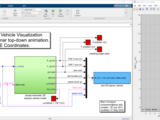
This Simulink model solves for the fixed terrain frame's XY position of the simple kinematic vehicle motion and visualizes the result using Matlab graphics. The Simulink model's base simulation timestep is h_fixed=0.05(s), or 50ms. On a 2Ghz Dell Inspiron laptop this model achieves near real-time operation at animation frame rates of 20fps to 30fps.
The Ackermann steering relationship delta_Ack = L / R is an approximation for a vehicle of wheelbase length L and track width W turning without slipping on a constant radius circle.
The Ackermann relationships are presented in Gillespie's 1992 text on page 186, Milliken and Milliken's 1995 text on page 128, or Wong's 2008 text page. 364. However none of these text's adequately and succinctly summarize the body-fixed velocity transformed into inertial, or terrain-fixed SAE XY coordinates. The handwritten notes provided here summarize the complete kinematic equation development.
Body-fixed SAE coordinates use +x pointing out the vehicle's front, +y out the passenger-side window, and +z down, into the ground. Terrain frame SAE XY coordinates have Z pointing downward into the ground.
Software Versions Tested:
-------------------------
This model was developed and tested using Matlab R2014 through R2020a and should work with any version. The animation s-function is a modified version of the level 1 m-file s-function from the Mathworks example provided in sanim.m.
Writing .jpeg animation frames to disk at each animation interval slows the simulation considerably. Set animation frames per second, anim_fps, in setup.m and re-run setup.m. Don't forget to turn off your file synchronization services to avoid syncing all the new image files.
Getting started:
-------------------------
Get started by unzipping the .zip file, changing directories to the folder, then running setup.m at the Matlb command prompt.
This will clear the workspace then populate it with the necessary variables to run the Simulink model and associated animation. It will also open the Simulink model file. Press Play or Simulation | Run to execute the Simulink model. The light blue s-function block will bring up the 2D animation figure window and display the steering vehicle at anim_fps frames per second.
-------------------------------------------------------------------------------
Distribution file list:
-------------------------------------------------------------------------------
[00_Readme.mdc.txt] - this file
[setup.m] - run this first, it will bring up the Simulink, then press play to simulate the vehicle
[createAviMovieFromAnimationSequence.m] - auxiliary m-file script for converting a sequence of .jpg images into an Avi using Matlab's VideoWriter() function.
[graphical_development.m] - auxiliary m-file script useful for developing the s-function graphics
[sanim_XY_vehicle_viz.m] - Simulink m-file s-function that displays Matlab graphics objects each animation interval (set by anim_fps in setup.m) to create the animation.
[veh_object2.m] - supporting m-file function to create vertices and faces for vehicle and tire graphics objects
[vehicle_animation_sim.png] - desktop screenshot showing the Simulink model and animation window
[vehicle_animation_sim.pdf] - printout of the Simulink block diagram in case you cannot open the Simulink
[vehicle_animation_sim.slx] - Matlab/Simulink R2020a model that expressed non-holonomically constrained (rolling) CG velocities and solves for vehicle position as a function of time.
[vehicle_animation_sim.mdl] - Matlab/Simulink R2013a model exported from R2020a using 'Export model to previous version of Simulink'
[.\anim_sequences] - folder where animation frame sequence .jpg files are stored; change this in sanim_XY_vehicle_viz.m
[.\Documentation\01_Lecture_A Simple 2D Kinematic Steering Model.pdf] - brief description of the model and interesting results with animation traces from points 'o' and 'g'.
[.\Documentation\02_Compere_handwritten_notes_kinematic_2D_vehicle_steering_model_Dec_2015,b.pdf] - Compere's handwritten notes with equations suitable for determining position of a steered vehicle in the terrain-fixed XY frame.
[.\Documentation\03_Compere_handwritten_notes_2D_Patch_Vehicle_and_Tire_Objects_Dec_2015.pdf] - example struture for defining Matlab handle graphics patch object faces and vertices, see veh_object2.m for implementation
-------------------------------------------------------------------------------
Textbook references:
-------------------------------------------------------------------------------
(1) Thomas Gillespie, Fundamentals of Vehicle Dynamics, SAE, 1992
(2) Milliken and Milliken, Race Car Vehicle Dynamics, SAE, 2005
(3) J. Y. Wong, Theory of Ground Vehicles, 4th Ed., Wiley, 2008
-----------------------------------
Marc Compere, comperem@erau.edu
created : 11 Jan 2016
modified: 16 Feb 2024
-----------------------------------

