Optimizing Performance and Fuel Economy of a Dual-Clutch Transmission Powertrain with Model-Based Design
By Pete Maloney, MathWorks and Wit Nursilo, MathWorks
Tight vehicle emission regulations and high fuel prices have intensified the demand for fuel-efficient cars. At the same time, customers continue to expect the same vehicle performance that they had when fuel prices were lower. These conflicting demands present an optimization challenge for automotive manufacturers: how to minimize fuel consumption and CO2 emissions without sacrificing performance?
In the distant past, automobile manufacturers tackled the problem by optimizing the power efficiency of each powertrain component separately. During the 1970s fuel crisis, large automakers began developing in-house computer simulation models to achieve optimal system-level performance. Despite this move toward system-level optimization, it is still common in some emerging markets to optimize individual components. This piecemeal approach misses a large opportunity to reduce vehicle-level fuel consumption by coordinating the operating points of the components.
Model-Based Design with MATLAB® and Simulink® enables all automakers and suppliers to achieve optimization results once reserved for a few large automakers with the resources to develop large internal simulation models and optimization programs. By using a system model that incorporates the engine, transmission, axle ratio, driver, and vehicle, engineers can precisely match powertrain components and optimize hardware variables, such as axle ratios, and calibration parameters, such as shift schedules, simultaneously. Instead of rough estimates of fuel economy impact derived from expensive technology alternatives, they then have hard metrics upon which to base crucial hardware-selection decisions.
For example, suppose we want to optimize the powertrain for an economy car with a five-speed, dual-clutch transmission (DCT) and a turbo-charged, 2-liter, 4-cylinder engine (Table 1). The goal is to use as little fuel as possible over a Federal Test Procedure (FTP75) drive cycle while maintaining a minimum performance threshold of 10 seconds for the 0–100 kph acceleration time (the time it takes to reach 100 kph from a standing start).
| Engine | Turbocharged 2.0L 4-cylinder I4 SI engine with dual-VVT |
| Vehicle class (mass) | Small to midsize (1600kg) |
| Transmission | 5-speed DCT |
| Drag coefficient Cd | 0.4 |
| Drive cycles | FTP75 (fuel economy) 0–100 kph acceleration (performance) |
Table 1. Vehicle characteristics.
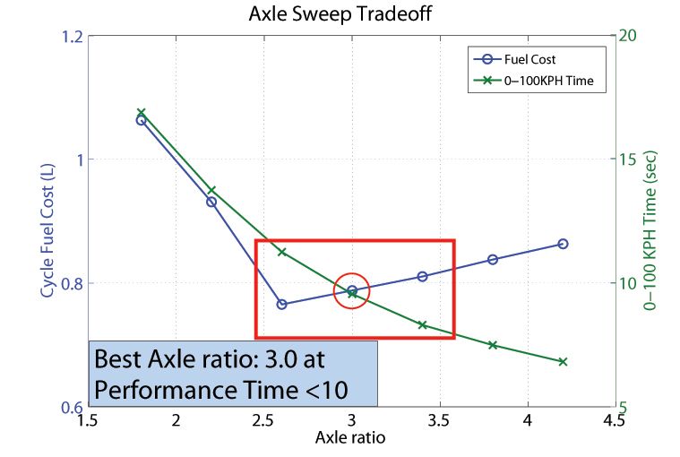
To find the combination of gear shift schedule calibrations and axle ratio that meets these requirements, we test a range of axle ratios. For each ratio, we use numerical optimization to find the most fuel-efficient shift schedule calibration for the FTP75 cycle, as well as a separate shift schedule calibration that minimizes 0–100 kph acceleration time. In keeping with current practice, the production powertrain controller chooses which of the two optimal shift schedules to use depending upon the magnitude of the torque demand sent by the driver through the accelerator pedal. Fuel cost and 0–100 kph acceleration time corresponding to each axle ratio are then plotted together to form a tradeoff graph of fuel economy and performance vs. axle ratio (Figure 1).
Instead of using expensive and time-consuming in-vehicle testing with axle hardware changes and shift-schedule recalibration, which can produce inconclusive results due to measurement noise, we now have a definitive result: Given a 10-second 0–100 kph design constraint, an axle ratio of 3.0 in combination with an optimal shift schedule calibration provides the best fuel efficiency.
Why DCT?
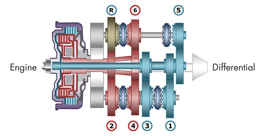
A DCT combines the convenience of an automatic transmission with the fuel efficiency of a manual transmission. It houses two separate clutches, one for odd and one for even gear sets (Figure 2), eliminating the need for a torque converter. To ensure smooth shifting and optimal efficiency, DCTs need sophisticated controllers capable of preselecting the next gear and engaging the appropriate clutch precisely when required.
DCTs are 3–5% more fuel-efficient than manual transmissions, which in turn are 5–10% more efficient than automatic transmissions. This efficiency gain has contributed to the recent growth of the DCT market, particularly in Europe and China.
Developing the System-Level Model
Working in Simulink, we build a system-level model that includes an accurate engine model derived from engine mapping data, the DCT (including its controller), the vehicle, and an autodriver component to drive the simulation through a specific drive cycle (Figure 3).
Engine Modeling and Calibration
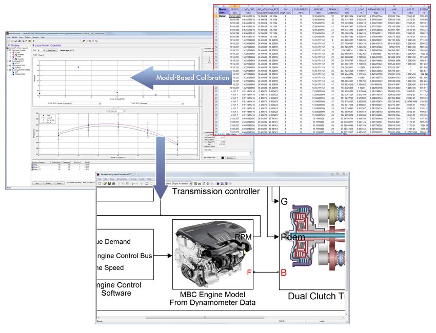
Since the engine is the heart of a conventional powertrain and directly consumes fuel, an accurate model of engine fuel consumption and torque production is crucial. To get the most accurate results, we must create this model from measured data. Using Model-Based Calibration Toolbox™ we fit statistical models to engine test data from an engine dynamometer and export those models automatically into Simulink (Figure 4).
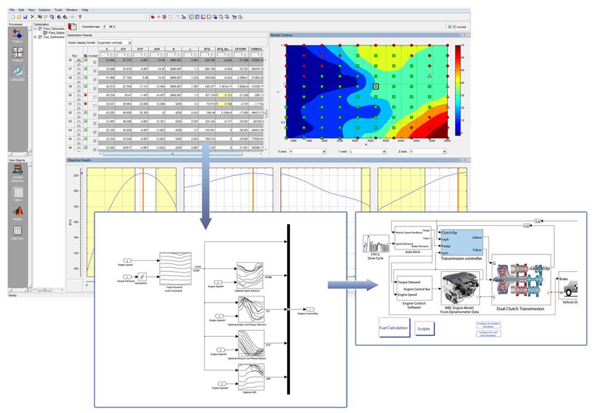
Using the Calibration Generation (CAGE) tool in Model-Based Calibration Toolbox, we generate engine calibration tables for use in the engine controller model of the overall simulation. These tables capture optimal spark advance, air-fuel ratio, intake cam phasing, and exhaust phasing as a function of engine speed and load (Figure 5).
Transmission and Vehicle Modeling
We model the DCT using actuator, dog clutch, gear, and shaft blocks from SimDriveline™ (as shown in the Simulink system model in Figure 3). The transmission controller, which includes the fuel economy and performance shift schedules, is modeled using Simulink and Stateflow®.
We also use SimDriveline to model a vehicle dynamics subsystem that incorporates the vehicle's mass and road-load characteristics.
Drive Cycle and Autodriver Implementation
To complete the system-level model, we add the FTP75 drive cycle and the autodriver subsystems. The FTP75 block incorporates the vehicle speed trace representing the standard Federal Test Procedure 75 drive cycle, which includes a mix of low- and mid-speed driving and is typically used for fuel economy and emission certification testing. The autodriver takes as input the vehicle speed command from the FTP75 block and the actual vehicle speed. It uses a proportional-integral (PI) controller to produce a torque demand signal that commands engine torque so that the actual vehicle speed matches the commanded vehicle speed from the FTP75 drive cycle.
Simulation and Optimization
Once we have a complete system-level model, we can run a simulation for any shift schedule and axle ratio that we want to test. The total fuel consumed and the 0–100 kph time can be calculated by the simulation.
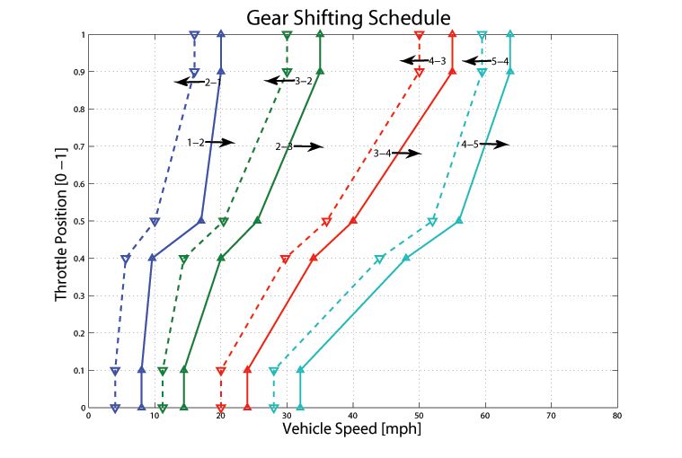
We will test seven axle ratios, ranging from 1.75 to 4.25, and determine the optimal gear shift schedule for each. A search that simulates every possible shift schedule is not feasible because the shift schedule comprises 32 different parameters (Figure 6). Assuming that each shift schedule calibration value can be varied over a range of +/-10 mph at an engineering resolution of 1 mph (not accounting for constraints), an exhaustive search would require the investigation of 2.05 x 1042 (2132) possible shift schedule simulations.
Instead of this brute force approach, we will use the pattern search optimization algorithm in Global Optimization Toolbox, reducing the number of simulations required—in this example, to 15,400.
An individual simulation of the FTP75 cycle takes only 250 seconds—about 5 times faster than real time. However, an optimization requiring 15,400 simulation runs on a single processor would take more than 44 days to get a result. This computationally intensive problem is a good candidate for parallel computing because the simulations can be run independently on separate processors.
We set up a computing cluster with 16 quad-core PCs, for a total of 64 workers. To further accelerate the search, we build a standalone executable target using Rapid Accelerator mode in Simulink to maintain complete simulation model parameter independence between runs.
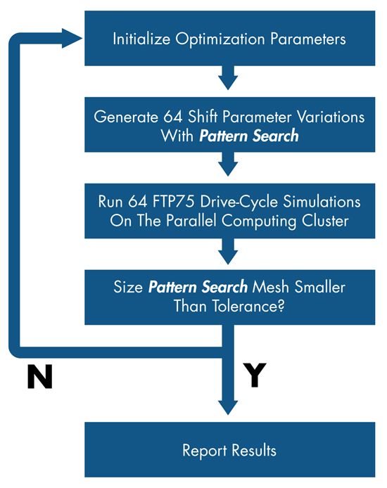
We begin the optimization process (Figure 7) by setting up the optimization parameters. Next, the pattern search algorithm in Global Optimization Toolbox identifies the parameter variations to be simulated using the 2N optimization method of pattern search. In this example there are two shift schedules, each with 16 variable points (N=32). This means that pattern search will run 64 (2N) simulations at a time, perfectly matching the number of workers available. Each variation is simulated for the current axle ratio on a different processor in the cluster. If the search space resolution, or mesh size, does not fall below a predetermined threshold, then a new set of parameter variations is generated and the process repeats. When the search space mesh size falls below the threshold, the algorithm has located a global minimum in fuel consumption of 0–100 kph time, and the results are reported.
Distributing this process on a 64-worker cluster reduces the total computation time from more than 44 days to about 26 hours.
After running a complete axle sweep and finding the optimal shift schedule for each axle ratio, we generate the performance and fuel economy tradeoff plot shown in Figure 1. The results show that the lowest fuel consumption is found at an axle ratio of about 2.6. This ratio, however, results in a 0–100 kph time of more than 10 seconds—above our 10-second performance threshold for the target market of the vehicle we are designing. The optimal axle ratio that falls below our desired performance threshold is 3.0.
Before running the optimization, we estimated an optimal shift schedule and axle ratio. This baseline configuration, with an axle ratio of 3.8, resulted in a vehicle fuel efficiency of 31.85 mpg and a 0–100 kph time of 8.03 seconds (Table 2). After running the optimization to find the most fuel-efficient shift schedule for this axle ratio, we increased fuel efficiency by 5.8%. By reducing the axle ratio to 3.0, we can trade off performance (0–100 kph time increases from 8.03 to 9.54) to achieve a fuel efficiency increase of 12.5% over the baseline.
If we had changed the axle ratio to 3.0 in a manual process without also reoptimizing the shift schedule, we would not have achieved the maximum possible fuel consumption reduction because it would have been difficult or impossible to adjust all 32 shift points manually to achieve the same result.
| Shift Schedule | Base | Opt 3.8 | Opt 3.0 |
| Axle Ratio | 3.8 | 3.8 | 3.0 |
| MPG | 31.85 | 5.8%↑ | 12.5%↑ |
| Performance Time 0–100 kph (s) |
8.03 | 8.03 | 9.54 |
Conclusions
Accurate vehicle simulation models enable engineers to quantitatively determine the optimal tradeoff between the conflicting demands of vehicle performance and fuel economy given a set of available hardware choices.
By using the approach described in this article, engineers can continue to respond to evolving market demands, changing the drivetrain axle ratio to select a tradeoff that matches customer expectations for a given class of vehicle.
Published 2011 - 91968v00

